Flux Balance Analysis of E. coli Central Carbon Metabolism: A Comprehensive Guide for Systems Biology and Metabolic Engineering
This article provides a comprehensive resource for researchers and scientists on applying Flux Balance Analysis (FBA) to Escherichia coli's central carbon metabolism (CCM).
Flux Balance Analysis of E. coli Central Carbon Metabolism: A Comprehensive Guide for Systems Biology and Metabolic Engineering
Abstract
This article provides a comprehensive resource for researchers and scientists on applying Flux Balance Analysis (FBA) to Escherichia coli's central carbon metabolism (CCM). It covers foundational principles, including the structure of CCM and its role in energy and precursor synthesis. The guide details core methodological approaches like constraint-based modeling and 13C-Metabolic Flux Analysis (13C-MFA) for experimental flux estimation. It further addresses advanced strategies for troubleshooting and optimizing models, such as integrating regulatory constraints and introducing synthetic pathways. Finally, the article outlines rigorous model validation and comparative analysis techniques to ensure predictive reliability. By synthesizing current methodologies and applications, this resource aims to enhance the use of E. coli in biotechnological and biomedical research, from rational strain design to drug development.
Understanding E. coli Central Carbon Metabolism: Network Structure and Functional Principles
Central carbon metabolism, comprising the core pathways of glycolysis, the pentose phosphate pathway (PPP), and the tricarboxylic acid (TCA) cycle, serves as the fundamental biochemical network for energy production and precursor generation in living organisms. In Escherichia coli, these pathways are not only conserved but have become a model system for quantitative analysis using techniques like Flux Balance Analysis (FBA) and kinetic modeling [1] [2]. These computational approaches allow researchers to interpret and predict metabolic phenotypes, understand the effects of genetic modifications, and identify critical regulatory nodes under various physiological conditions, including oxidative stress and overflow metabolism [3] [4]. This guide provides an in-depth technical overview of these core pathways, detailing their reactions, quantitative flux distributions, and the experimental and computational methodologies essential for studying them within the context of E. coli central carbon metabolism.
Glycolysis (Embden-Meyerhof-Parnas Pathway)
Glycolysis is a ten-step metabolic sequence that converts one molecule of glucose into two molecules of pyruvate, yielding a net gain of ATP and NADH [1] [5]. In E. coli, glucose is often transported into the cell via the Phosphotransferase System (PTS), which simultaneously phosphorylates it to Glucose-6-Phosphate (G6P) [1]. The key enzymes include phosphofructokinase (Pfk), a highly regulated step, and pyruvate kinase (Pyk), which catalyzes the final yield of pyruvate [1].
Pentose Phosphate Pathway (PPP)
The PPP operates in two distinct phases: the oxidative and non-oxidative branches. The oxidative phase, starting with G6P, is a primary source of cellular NADPH, essential for reductive biosynthesis and oxidative stress response [3]. The non-oxidative phase involves a series of carbon-shuffling reactions, catalyzed by transketolases and transaldolases, which generate various sugar phosphates like Ribose-5-Phosphate (R5P) for nucleotide synthesis and link back to glycolytic intermediates [1] [3].
Tricarboxylic Acid (TCA) Cycle and Associated Pathways
The TCA cycle is the central hub for the aerobic oxidation of acetyl-CoA, derived from pyruvate, producing NADH, FADH2, and GTP, as well as precursor molecules for biosynthesis [1]. In E. coli, the cycle is closely integrated with the glyoxylate shunt and anaplerotic reactions [1]. The glyoxylate shunt, bypassing decarboxylative steps in the TCA cycle, allows for the net assimilation of carbon from two-carbon compounds like acetate [1]. Anaplerotic reactions, such as those catalyzed by phosphoenolpyruvate carboxylase (Ppc) and malic enzyme (Mez), replenish TCA cycle intermediates drawn off for biosynthesis [1] [3].
Table 1: Key Metabolic Reactions in E. coli Central Carbon Metabolism
| Pathway | Reaction/Step Abbreviation | Enzyme | Input | Output |
|---|---|---|---|---|
| Glycolysis | Pgi | Phosphoglucose isomerase | Glucose-6-Phosphate (G6P) | Fructose-6-Phosphate (F6P) |
| Pfk | Phosphofructokinase | Fructose-6-Phosphate (F6P) | Fructose-1,6-bisphosphate (FDP) | |
| Pyk | Pyruvate kinase | Phosphoenolpyruvate (PEP) | Pyruvate (PYR) | |
| PPP | G6pdh | Glucose-6-phosphate dehydrogenase | Glucose-6-Phosphate (G6P) | NADPH + 6-Phosphogluconolactone |
| Gnd | 6-Phosphogluconate dehydrogenase | 6-Phosphogluconate | NADPH + Ribulose-5-Phosphate | |
| Tkt | Transketolase | Various sugar phosphates | Various sugar phosphates | |
| TCA Cycle | Glta | Citrate synthase | Acetyl-CoA + Oxaloacetate (OAA) | Citrate (CIT) |
| Icd | Isocitrate dehydrogenase | Isocitrate (ICIT) | NADPH + α-Ketoglutarate (AKG) | |
| Akd | α-Ketoglutarate dehydrogenase | α-Ketoglutarate (AKG) | NADH + Succinyl-CoA | |
| Sdh | Succinate dehydrogenase | Succinate | FADH2 + Fumarate | |
| Mdh | Malate dehydrogenase | Malate | NADH + Oxaloacetate (OAA) | |
| Glyoxylate Shunt | AceA | Isocitrate lyase | Isocitrate (ICIT) | Glyoxylate + Succinate |
| AceB | Malate synthase | Glyoxylate + Acetyl-CoA | Malate | |
| Anaplerotic | Ppc | Phosphoenolpyruvate carboxylase | Phosphoenolpyruvate (PEP) | Oxaloacetate (OAA) |
| Mez | Malic enzyme | Malate | NADPH + Pyruvate (PYR) |
Metabolic Flux Analysis and Quantitative Flux Distributions
Metabolic flux is defined as the in vivo rate of an enzyme reaction, representing the number of converted molecules per unit time per cell (mol h⁻¹ cell⁻¹) [5]. It is the definitive parameter for investigating cell metabolism because the activation and inactivation of metabolic pathways can be directly evaluated by determining flux levels. Flux Balance Analysis (FBA) is a constraint-based modeling approach used to compute the flow of metabolites through a metabolic network [2]. It relies on solving a system of linear equations based on the stoichiometric matrix (S) of all reactions, subject to mass balance constraints (S • v = 0, where v is the flux vector) and capacity constraints (αᵢ ≤ vᵢ ≤ βᵢ) [2]. FBA can predict optimal flux distributions that maximize a cellular objective, typically biomass production, and has been successfully used to interpret the metabolic phenotypes of wild-type and mutant E. coli strains [2].
Table 2: Experimentally Determined Metabolic Fluxes in E. coli Central Metabolism (mmol g⁻¹ h⁻¹) [3]
| Metabolic Flux | Normal Medium | PQ-containing Medium (Oxidative Stress) | Notes |
|---|---|---|---|
| Specific α-Ketoglutarate Production (Qakg) | 0.84 ± 0.13 | 1.73 ± 0.18 | More than doubles under stress |
| Specific Pyruvate Production (Qpyr) | 0.04 ± 0.005 | 0.02 ± 0.008 | Decreases under stress |
| Specific Lactate Production (Qlac) | 0.32 ± 0.05 | 0.21 ± 0.06 | Decreases under stress |
| Specific Acetate Production (Qace) | - | 4.31 ± 1.2 | Significant production induced |
| Biomass Yield on Glucose (Ybiomass/glc) | 0.37 ± 0.03 | 0.322 ± 0.023 | Reduced yield under stress |
| NADPH:NADH Ratio | ~0.81 | ~1.15 (Increase of 1.6-1.8x) | Measured and calculated from fluxes |
Quantitative flux analyses have revealed how E. coli redistributes its metabolism in response to environmental challenges. For instance, under paraquat-induced superoxide stress, fluxes are systematically redirected [3]:
- PPP fluxes increase to generate more NADPH for antioxidant defense.
- TCA cycle fluxes (e.g., Icd, Akd) decrease, while the glyoxylate shunt fluxes increase.
- Acetate efflux increases significantly, a phenomenon known as overflow metabolism [4].
Experimental Protocols and Methodologies
¹³C-Metabolic Flux Analysis (¹³C-MFA)
¹³C-MFA is a powerful method for estimating the in vivo flux distribution in central carbon metabolism from experimentally measured specific rates and ¹³C-labeling patterns of metabolites under metabolic steady state [5].
Protocol Summary:
- Cultivation: Grow E. coli in a controlled bioreactor (e.g., chemostat) with a defined medium where the sole carbon source (e.g., glucose) is replaced with a ¹³C-labeled variant (e.g., [1-¹³C]-glucose or [U-¹³C]-glucose) [3] [5].
- Metabolite Extraction: At metabolic steady-state, rapidly sample the culture and quench metabolism (e.g., using cold methanol). Intracellular metabolites are extracted [5].
- Mass Spectrometry (GC-MS) Analysis: Derivatize the metabolite extracts and analyze them using Gas Chromatography-Mass Spectrometry (GC-MS). The mass isotopomer distributions (MIDs) of the fragments are measured [5].
- Flux Calculation: Use specialized software (e.g., ¹³C-FLUX) to integrate the measured MIDs with the stoichiometric model of the metabolic network. The software performs parameter fitting to find the flux map that best reproduces the experimental labeling data [3]. Confidence intervals for the estimated fluxes can be calculated using statistical methods like Monte Carlo sampling [3].
Kinetic Model Construction and Parameter Estimation
Kinetic models simulate the dynamic behavior of metabolic pathways by using enzyme rate equations, which require knowledge of kinetic parameters [1].
Protocol Summary:
- Network Definition: Construct a detailed map of the metabolic network, including all relevant reactions, allosteric effectors, and gene regulatory interactions (e.g., by transcription factors like Crp, Cra) [1].
- Rate Equation Formulation: Assign appropriate kinetic rate laws (e.g., Michaelis-Menten, Hill equations) to each enzymatic reaction based on literature [1].
- Parameter Estimation: Use computational optimization algorithms (e.g., genetic algorithms) on high-performance computing systems to estimate the unknown kinetic parameter values. The objective is to minimize the difference between model simulations and experimental time-course data (e.g., biomass, extracellular metabolites, intracellular metabolite concentrations) [1].
- Model Validation: Validate the model by testing its ability to accurately reproduce the dynamic behavior of wild-type E. coli and, crucially, various genetic knockout mutants (e.g., ∆pykF, ∆pgi) in a batch culture [1].
Visualization of Metabolic Networks and Analysis Workflows
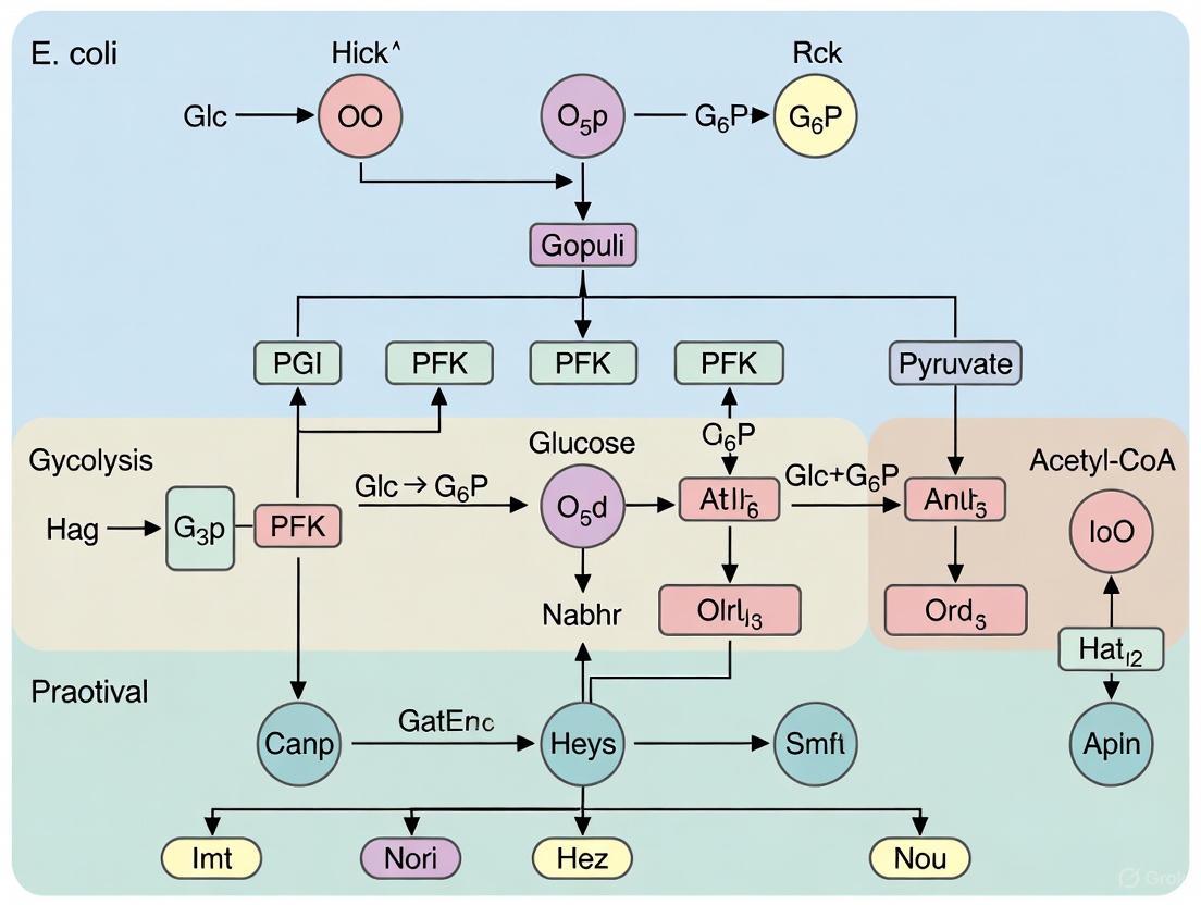
E. coli Central Carbon Metabolic Network
Diagram 1: E. coli Central Carbon Metabolic Network. The diagram shows the integration of glycolysis, PPP, TCA cycle, glyoxylate shunt (green), and anaplerotic reactions (yellow). NADPH-producing reactions are highlighted in red.
¹³C-MFA Experimental Workflow
Diagram 2: ¹³C-MFA Experimental Workflow. Key steps from cultivating cells with a labeled carbon source to generating a statistically validated quantitative flux map.
The Scientist's Toolkit: Essential Research Reagents and Materials
Table 3: Key Research Reagent Solutions for Central Metabolism Studies
| Reagent/Material | Function and Application | Example Use Case |
|---|---|---|
| ¹³C-Labeled Glucose (e.g., [1-¹³C], [U-¹³C]) | Tracer for ¹³C-MFA; allows for the experimental determination of intracellular metabolic fluxes by incorporating a measurable isotopic label into metabolites. | Used in chemostat cultivations to trace the fate of carbon atoms through the metabolic network and quantify flux distributions [3] [5]. |
| Enzyme Activity Assay Kits | In vitro measurement of the maximum catalytic activity (Vmax) of specific enzymes (e.g., G6PDH, AKGDH). | Used to validate changes in enzyme capacity suggested by flux or gene expression data, particularly in response to stressors like paraquat [3]. |
| Metabolite Standards (LC-MS/GC-MS grade) | Absolute quantification of intracellular metabolite concentrations (metabolomics) using mass spectrometry. | Essential for calculating Gibbs free-energy changes (ΔG') of reactions and evaluating the thermodynamic state of pathways [5]. |
| Paraquat (Methyl Viologen) | Chemical inducer of superoxide stress; used to perturb the metabolic network and study the resulting flux adaptations. | Applied in chemostat studies to investigate the redox stress response, including flux rerouting to the PPP [3]. |
| Stoichiometric Model (e.g., iML1515) | A computational matrix (S) representing all known metabolic reactions in E. coli. The core constraint for FBA. | Used in FBA and ¹³C-MFA to simulate metabolic behavior and interpret mutant phenotypes in silico [2]. |
| Kinetic Model Parameters (Kₘ, kcat, Hill coeff.) | Experimentally derived or fitted constants for enzyme rate equations. Enable dynamic simulation of metabolism. | Estimated via optimization algorithms to build predictive kinetic models of the central metabolic network [1]. |
The Role of CCM in Energy Production, Redox Balancing, and Biomass Precursor Synthesis
Central Carbon Metabolism (CCM) serves as the biochemical core of Escherichia coli, integrating catabolic and anabolic processes to sustain cellular life. This network encompasses the primary pathways responsible for energy production, redox balancing, and the synthesis of critical biomass precursors. In the context of metabolic engineering and flux balance analysis (FBA) research, a detailed understanding of CCM is paramount for manipulating bacterial physiology for biomedical and biotechnological applications. The recent development of curated metabolic models like iCH360, a manually refined sub-network of the genome-scale iML1515 reconstruction, provides an optimized framework for investigating these processes with enhanced biological accuracy [6]. These models facilitate sophisticated computational analyses, including enzyme-constrained FBA and thermodynamic profiling, enabling researchers to predict intracellular flux distributions and identify key regulatory nodes under various genetic and environmental conditions.
The functional output of CCM is fundamentally governed by its architectural properties. The E. coli metabolic network, as cataloged in foundational resources like EcoCyc, comprises hundreds of interconnected reactions and metabolites [7]. CCM demonstrates remarkable robustness, maintaining flux ratio homeostasis despite significant genetic perturbations, such as the overexpression of key enzymes like phosphofructokinase or pyruvate kinase [8]. This inherent stability underscores the complexity of its regulatory design. For drug development professionals, targeting this metabolic network offers promising avenues for disrupting bacterial viability. This guide provides a technical examination of CCM, consolidating quantitative data, experimental protocols, and visual tools to support advanced research in this field.
Quantitative Architecture ofE. coliCCM
The global properties of the E. coli metabolic network reveal a system optimized for efficiency and connectivity. Computational analyses of the EcoCyc database quantify the network as consisting of 744 reactions catalyzed by 607 enzymes, which act upon 791 distinct chemical substrates [7]. This network is organized into 131 pathways, with pathway lengths ranging from single-step reactions to extended sequences of up to 16 steps, averaging 5.4 reactions per pathway [7].
Key Metabolite Participation Frequencies
The connectivity of the network is underscored by the recurrence of specific metabolites across numerous reactions. The following table lists the most frequently occurring substrates in E. coli small-molecule metabolism, highlighting the central role of energy carriers, redox cofactors, and universal metabolites [7].
Table 1: High-Frequency Metabolites in E. coli Central Carbon Metabolism
| Metabolite | Number of Reactions | Primary Metabolic Role |
|---|---|---|
| H₂O | 205 | Universal solvent, hydrolysis/hydration reactions |
| ATP | 152 | Primary energy currency, phosphorylation |
| ADP | 101 | Energy regeneration, product of ATP hydrolysis |
| Phosphate | 100 | Phosphorylation, energy transfer |
| Pyrophosphate | 89 | Biosynthetic reactions, driving irreversible steps |
| NAD | 66 | Redox cofactor (oxidized form), electron acceptor |
| NADH | 60 | Redox cofactor (reduced form), electron donor |
| CO₂ | 54 | Product of decarboxylation reactions, gas |
| H⁺ | 53 | Proton, pH regulation, chemiosmotic energy |
| AMP | 49 | Energy status indicator, allosteric regulation |
Functional Organization of Metabolic Pathways
The pathways of CCM can be categorized based on their primary functional outputs. The table below summarizes the core pathways directly involved in energy production, redox balancing, and the synthesis of biomass precursors.
Table 2: Core Functional Pathways in E. coli Central Carbon Metabolism
| Pathway Name | Primary Function | Key Inputs | Key Outputs |
|---|---|---|---|
| Glycolysis (Embden-Meyerhof-Parnas) | Glucose catabolism, net ATP/NADH production, precursor generation | Glucose, ATP, NAD⁺ | Pyruvate, ATP, NADH, Precursors (G3P, PEP) |
| Tricarboxylic Acid (TCA) Cycle | Complete oxidation of acetyl-CoA, high-yield NADH/FADH₂ generation, precursor provision | Acetyl-CoA, Oxaloacetate, NAD⁺, GDP | CO₂, NADH, FADH₂, ATP (GTP), Biosynthetic precursors |
| Pentose Phosphate Pathway (PPP) | NADPH production for biosynthesis, pentose sugars for nucleotides | Glucose-6-P, NADP⁺ | Ribose-5-P, NADPH, CO₂ |
| Oxidative Phosphorylation | ATP synthesis via proton motive force, redox balancing (NADH/FADH₂ oxidation) | NADH, FADH₂, O₂ (terminal e⁻ acceptor), ADP + Pi | ATP, H₂O, NAD⁺, FAD |
| Gluconeogenesis | Glucose synthesis from non-carbohydrate precursors | Pyruvate, Oxaloacetate, ATP | Glucose-6-P |
| Glyoxylate Shunt | Anaplerotic pathway for TCA cycle during growth on C₂ substrates (e.g., acetate) | Acetyl-CoA, Glyoxylate | Succinate, Malate |
Experimental Analysis of Metabolic Flux
Metabolic Flux Ratio (METAFoR) Analysis
Principle: METAFoR analysis is a powerful methodology that determines the relative fluxes of converging metabolic pathways and identifies active routes in central carbon metabolism. It is based on two-dimensional ¹³C-¹H correlation nuclear magnetic resonance (NMR) spectroscopy of hydrolyzed cell protein from biomass that has been fractionally labeled with [U-¹³C₆]glucose [8]. The technique leverages the fact that alternative metabolic pathways produce different patterns of intact carbon-carbon bonds from a single glucose molecule, which are then preserved in the amino acids of cellular protein.
Workflow Diagram:
Diagram Title: METAFoR Analysis Experimental Workflow
Detailed Protocol:
Strain and Medium Preparation:
- Utilize E. coli strains such as the wild-type K-12 strain MG1655 or other relevant derivatives (e.g., JM101, PB25) [8].
- Prepare a defined minimal medium. A standard composition per liter includes [8]:
- 5 g Glucose (for batch culture)
- 48 mM Na₂HPO₄
- 22 mM KH₂PO₄
- 10 mM NaCl
- 30 mM (NH₄)₂SO₄
- 1 mM MgSO₄ (separately sterilized)
- 0.1 mM CaCl₂ (separately sterilized)
- 1 mg Vitamin B₁ (Thiamine) (filter sterilized)
- 10 mL Trace element solution
Fractional Labeling and Cultivation:
- Replace natural abundance glucose in the medium with a mixture of 85-90% natural abundance glucose and 10-15% [U-¹³C₆]glucose (¹³C, >98%) [8].
- Inoculate the medium and grow cells under controlled conditions (e.g., 30°C for aerobic batch cultures in baffled shake flasks at 200 rpm). For chemostat studies, operate at a steady state (e.g., dilution rate D = 0.2 h⁻¹) before switching to the labeled feed.
Biomass Harvesting and Processing:
- Harvest biomass during mid-exponential growth phase (or after one volume change in chemostats to ensure ~63% fractional labeling).
- Centrifuge cells, wash, and lyse.
- Hydrolyze the harvested cellular protein using 6 M HCl at 105°C for 24 hours to release free amino acids [8].
NMR Spectroscopy and Data Analysis:
- Analyze the hydrolyzed amino acid mixture using two-dimensional ¹³C-¹H correlation NMR (COSY).
- Quantify the intensities of the multiplet components in the ¹³C fine structure of specific amino acid carbon atoms. These multiplets reflect the relative abundance of intact carbon fragments from the original glucose.
- Apply probabilistic equations to the multiplet data to derive intracellular metabolic flux ratios, such as the fraction of phosphoenolpyruvate (PEP) molecules derived through transketolase reactions or the relative contribution of anaplerotic PEP carboxylation versus the TCA cycle for oxaloacetate synthesis [8].
Research Reagent Solutions
The following table details key reagents and computational tools essential for experimental and in silico analysis of E. coli CCM.
Table 3: Essential Research Reagents and Tools for CCM Analysis
| Reagent / Tool | Function / Purpose | Example & Context |
|---|---|---|
| [U-¹³C₆]glucose | Tracer for METAFoR analysis and ¹³C Metabolic Flux Analysis (MFA). | Enables determination of pathway fluxes and ratios via NMR or MS; used at 10-15% labeling fraction [8]. |
| Defined Minimal Medium | Provides controlled nutrient environment for physiological studies. | Essential for chemostat cultures and labeling experiments to avoid unaccounted carbon sources [8]. |
| iCH360 Metabolic Model | A manually curated, medium-scale model for constraint-based modeling of E. coli core and biosynthetic metabolism. | Used for Flux Balance Analysis (FBA), enzyme-constrained simulations, and EFM analysis; a sub-network of iML1515 [6]. |
| EcoCyc Database | Comprehensive, literature-based knowledgebase of E. coli genes, metabolism, and regulation. | Used for pathway information, gene-reaction associations, and biochemical data retrieval [9] [7]. |
| Fluxer Web Application | Tool for automated FBA computation and visualization of genome-scale metabolic models. | Visualizes flux distributions as spanning trees or dendrograms from SBML models; useful for interpreting FBA results [10]. |
Computational Modeling of CCM: Flux Balance Analysis
Fundamentals and Application of FBA
Flux Balance Analysis (FBA) is a constraint-based modeling approach used to predict the flow of metabolites through a metabolic network at steady state. It computes reaction rates (fluxes) that optimize a cellular objective, typically the maximization of biomass production, which represents bacterial growth [10]. The iCH360 model is particularly suited for this analysis as it retains the critical pathways for energy and precursor synthesis while being compact enough for advanced analyses like Elementary Flux Mode (EFM) analysis and thermodynamic profiling [6]. FBA can predict the outcome of genetic manipulations, such as gene knockouts, and environmental perturbations, providing testable hypotheses for experimental validation.
FBA Workflow and Pathway Integration
The following diagram illustrates the logical flow of FBA and how CCM pathways are integrated to achieve the core functions of energy production, redox balance, and biomass synthesis.
Diagram Title: FBA Logic and CCM Pathway Integration
The central carbon metabolism of E. coli is a highly integrated and robust system that efficiently coordinates energy production, redox homeostasis, and the generation of biomass precursors. The continued development of curated metabolic models like iCH360, coupled with advanced experimental techniques such as METAFoR analysis, provides an increasingly quantitative and mechanistic understanding of this system. The integration of rich biological data—including thermodynamic and kinetic parameters—into these models enhances their predictive power for both basic research and applied fields.
For drug development, targeting the unique aspects of bacterial CCM, especially under infection-relevant conditions like nutrient limitation, presents a promising strategy for novel antimicrobials. Furthermore, the principles of growth-coupled selection, where cell survival is linked to the activity of an engineered pathway, are being leveraged to rewire E. coli CCM for biotechnological applications, including the production of sustainable chemicals and materials [11]. Future research will focus on further refining models to capture regulatory constraints and on using these integrated computational and experimental approaches to precisely control metabolic flux for desired outcomes.
Principles of Constraint-Based Modeling and Steady-State Assumption in FBA
Flux Balance Analysis (FBA) is a mathematical approach for simulating metabolism of cells or entire unicellular organisms using genome-scale metabolic reconstructions [12]. This constraint-based modeling method has become a cornerstone of systems biology, enabling researchers to study metabolic network behavior without requiring extensive kinetic parameter data. FBA operates on the fundamental premise that stoichiometric, thermodynamic, and capacity constraints limit the flux values for biochemical reactions within a cell to a feasible region known as the solution space [13]. The method has found diverse applications in bioprocess engineering, drug target identification, culture media design, and host-pathogen interaction studies [12]. When applied to E. coli central carbon metabolism, FBA provides a powerful framework for predicting how genetic modifications or environmental changes affect metabolic flux distributions, enabling rational design of microbial cell factories for industrial biotechnology.
The steady-state assumption represents the core theoretical foundation of FBA, distinguishing it from dynamic modeling approaches that require detailed kinetic parameters [14] [15]. This principle posits that metabolite concentrations remain constant over the timescale of analysis, with production and consumption rates balanced to achieve no net accumulation or depletion of intracellular metabolites. For E. coli metabolism, this assumption is particularly relevant during balanced exponential growth, where internal metabolite pools remain relatively stable while biomass components are synthesized at constant rates.
Mathematical Foundations of FBA
Core Mathematical Formulation
The mathematical basis of FBA formalizes the system of equations describing metabolic concentration changes as the dot product of a stoichiometric matrix (S) and a flux vector (v), equaling zero at steady state [12]:
S ⋅ v = 0
This equation represents the mass balance constraint for all metabolites in the system. The stoichiometric matrix S is an m × n matrix where m represents the number of metabolites and n the number of reactions. Each element Sij corresponds to the stoichiometric coefficient of metabolite i in reaction j. The flux vector v contains the reaction rates (fluxes) through each metabolic reaction.
The underdetermined nature of this system (typically more reactions than metabolites) necessitates additional constraints to identify meaningful biological solutions:
lowerbound ≤ v ≤ upperbound
These inequality constraints implement reaction reversibility/irreversibility and capacity limits based on enzyme activity or substrate uptake rates.
Optimization Framework
FBA identifies a particular flux distribution from the feasible solution space by optimizing an objective function, typically formulated as a linear programming problem [12]:
where c is a vector of coefficients defining the linear objective function, with typically only one element (corresponding to biomass production) set to 1 and others to 0. For E. coli models, the biomass objective function often incorporates experimentally determined biomass composition data, representing the drain of biosynthetic precursors needed to support cellular growth.
The Steady-State Assumption: Theoretical Basis and Implications
Physiological Basis and Validity
The steady-state assumption in FBA reduces the system to a set of linear equations by asserting that internal metabolite concentrations do not change significantly during the analysis period [12]. This assumption is biologically justified for E. coli central carbon metabolism during mid-exponential growth in batch culture or in continuous culture at steady state, where metabolic fluxes remain relatively constant over time. The material balance model underlying this approach can be summarized as:
Input = Output + Accumulation
With the steady-state assumption, the accumulation term becomes zero, simplifying to:
Input - Output = 0
This simplification makes the analysis tractable for genome-scale models containing thousands of reactions and metabolites. The steady-state formulation has no mechanistic knowledge of chemical reactions beyond their stoichiometry and produces a high-dimensional continuum of steady-state solutions rather than a unique solution [14] [15].
Comparison with Dynamic Formulations
Dynamic models based on ordinary differential equations (ODEs) provide an alternative modeling approach that describes metabolite concentration changes over time using kinetic rate laws [14] [15]. These models contain detailed mechanistic information but require extensive parameter estimation. Comparative studies of E. coli central carbon metabolism have revealed that dynamic and constraint-based formulations describe the same set of steady states when unconstrained [14] [15]. However, incorporating partial kinetic parameter knowledge into dynamic models can generate additional constraints that reduce the solution space below that identified by constraint-based models alone, eliminating infeasible solutions [15].
Diagram 1: Relationship between modeling components showing how additional constraints reduce the feasible solution space.
Solution Space Analysis and Sampling Methods
Characterizing the Feasible Flux Space
The solution space of an FBA model comprises all flux distributions satisfying the stoichiometric and constraint equations [13]. This space forms a convex polyhedron in n-dimensional flux space. For realistic models, this space remains extensively underdetermined even after applying all constraints, resulting in infinite feasible flux distributions. Several approaches have been developed to characterize this space:
- Flux Variability Analysis (FVA): Determines the minimum and maximum possible flux for each reaction while maintaining optimal objective value [13]
- Solution Space Kernel (SSK): Identifies a bounded, low-dimensional kernel that facilitates geometric interpretation of the solution space [13]
- Extreme Pathway/Elementary Mode Analysis: Finds a vector basis that completely spans the solution space [13]
The SSK approach specifically addresses unbounded fluxes common in metabolic models by separating them into ray vectors and focusing on the bounded kernel containing biologically relevant flux ranges [13].
Sampling Methods for Solution Space Characterization
Multiple computational approaches have been developed to map the feasible steady-state flux space:
Hit-and-Run Sampler [14]:
- Starts with a point inside the coordinate space
- Generates new points by iterative steps in random directions
- Projects points into flux space and tests boundary constraints
- Implements variable step size for efficient sampling
Geometric Sampler [14]:
- Identifies flux cone corners using linear programming with randomized objective functions
- Samples along edges between corners to define cone boundaries
- Iteratively samples toward the center of the cone
- Facilitates visualization but lacks statistical meaning in probability distribution
Parameter Sampler for Dynamic Models [14]:
- Samples kinetic parameters and concentrations using log-normal distributions
- Enables mapping of allowed steady states in dynamic formulations
- Allows constrained parameter variation within defined ranges
Extensions and Refinements to Classical FBA
Incorporating Additional Biological Constraints
Table 1: Advanced FBA Formulations and Their Applications
| Method | Key Features | Applications in E. coli Metabolism | References |
|---|---|---|---|
| flexFBA | Removes fixed proportion between biomass reactants; allows independent production of process metabolites | Modeling metabolite production in non-wild-type proportions; single-cell modeling | [16] |
| tFBA | Removes fixed proportion between reactants and byproducts; enables transient behavior modeling | Simulating transitions between metabolic steady states; integrated whole-cell modeling | [16] |
| ECMpy | Incorporates enzyme constraints based on availability and catalytic efficiency | Capping unrealistic flux predictions; modeling engineered enzymes | [17] |
| DFBA | Combines FBA with differential equations for extracellular metabolites | Simulating batch processes; dynamic bioprocess optimization | [18] [19] |
| rFBA | Integrates regulatory constraints with metabolic networks | Predicting metabolic responses to genetic perturbations | [20] |
Hybrid Modeling Approaches
Recent advances have integrated machine learning with constraint-based models to enhance predictive power. Neural-mechanistic hybrid models embed FBA within artificial neural networks, enabling learning from flux distributions while respecting mechanistic constraints [21]. These approaches address a critical limitation of classical FBA: the conversion of medium composition to uptake fluxes [21]. The hybrid models require training set sizes orders of magnitude smaller than classical machine learning methods while systematically outperforming standard constraint-based models [21].
Diagram 2: Architecture of neural-mechanistic hybrid models showing integration of machine learning with FBA.
Experimental Protocols and Methodologies
Protocol for Implementing Enzyme-Constrained FBA
The ECMpy workflow provides a standardized approach for incorporating enzyme constraints into genome-scale metabolic models of E. coli [17]:
Model Preparation:
- Obtain a curated genome-scale model (e.g., iML1515 for E. coli K-12 MG1655)
- Split reversible reactions into forward and reverse reactions to assign direction-specific kcat values
- Separate reactions catalyzed by multiple isoenzymes into independent reactions
Parameter Acquisition:
- Calculate molecular weights using protein subunit composition from EcoCyc
- Obtain protein abundance data from PAXdb
- Acquire kcat values from BRENDA database
- Set protein mass fraction constraint (typically 0.56 for E. coli)
Implementation of Enzyme Constraints:
- Add total enzyme capacity constraint based on measured protein fraction
- Incorporate enzyme-specific constraints using kcat values and molecular weights
- Modify kinetic parameters to reflect engineered enzymes (e.g., SerA, CysE for L-cysteine production)
Simulation and Analysis:
- Perform FBA with lexicographic optimization (biomass growth followed by product formation)
- Conduct flux variability analysis to identify flexible reactions
- Compare predictions with experimental data
Protocol for Dynamic FBA Implementation
Dynamic FBA extends standard FBA to simulate time-dependent processes [18] [19]:
Initialization:
- Define initial biomass and extracellular metabolite concentrations
- Set uptake kinetic parameters for extracellular substrates
Time-Stepping Loop:
- Calculate current uptake bounds based on extracellular concentrations
- Solve FBA problem to determine intracellular fluxes and growth rate
- Update biomass using computed growth rate: dB/dt = μ·B
- Update extracellular metabolites using computed exchange fluxes: dC/dt = v_exchange·B
- Advance to next time step
Termination:
- Stop simulation when nutrients depleted or target time reached
- Output time courses of biomass, metabolites, and fluxes
This approach is particularly valuable for modeling E. coli fermentations where changing substrate concentrations significantly impact metabolic fluxes.
Research Reagent Solutions for FBA Studies
Table 2: Essential Research Reagents and Computational Tools for E. coli FBA
| Resource Type | Specific Examples | Function in FBA Research | Source/Reference |
|---|---|---|---|
| Genome-Scale Models | iML1515, EcoCyc-based reconstructions | Provides stoichiometric matrix for E. coli metabolism | [17] |
| Enzyme Kinetic Data | BRENDA database, UniKP predictions | Parameterizes enzyme-constrained models | [17] |
| Protein Abundance Data | PAXdb, experimental proteomics | Constrains total enzyme allocation | [17] |
| Software Tools | COBRApy, ECMpy, SSKernel | Implements FBA and solution space analysis | [13] [17] |
| Experimental Flux Data | 13C metabolic flux analysis | Validates FBA predictions | [14] |
| Media Composition Databases | LB, SM1, M9 minimal media | Defines uptake constraints for simulations | [17] |
Applications to E. coli Central Carbon Metabolism
Constraint-based modeling of E. coli central carbon metabolism has enabled numerous applications in metabolic engineering and basic research. Comparative analyses of dynamic and constraint-based formulations of the same E. coli central carbon model have demonstrated equivalence in their steady-state solution spaces when unconstrained [14] [15]. However, incorporating partial kinetic information allows dynamic models to generate additional constraints that reduce the solution space and eliminate infeasible solutions.
Implementation of enzyme constraints using the ECMpy workflow has proven particularly valuable for modeling engineered E. coli strains for L-cysteine production [17]. By modifying kcat values and gene abundance parameters to reflect mutant enzymes (SerA, CysE, EamB), researchers can more accurately predict metabolic fluxes and optimize production strategies. These approaches successfully address the common FBA limitation of predicting unrealistically high fluxes by accounting for enzyme availability and catalytic capacity.
The steady-state assumption remains central to all these applications, providing a tractable framework for analyzing complex metabolic networks while maintaining biological relevance for E. coli growing under constant conditions. Ongoing development of hybrid dynamic-constraint-based methods continues to expand the applicability of FBA to transient processes and changing environmental conditions.
Key Metabolite Hubs and Their Regulatory Roles in Flux Control
This technical guide examines the critical role of metabolite hubs in controlling metabolic flux within Escherichia coli central carbon metabolism. Metabolites function not merely as passive intermediates but as active regulators of flux through allosteric modulation, post-translational modification, and transcriptional regulation. Understanding these regulatory mechanisms is paramount for rational metabolic engineering and therapeutic intervention. Framed within the context of flux balance analysis (FBA) research, this review synthesizes contemporary insights into metabolite-protein interactions, quantitative flux control analysis, and computational frameworks for predicting flux distributions. We provide detailed methodologies for profiling metabolite interactions, summarize key regulatory metabolites in tabular form, and present essential research tools for investigating flux control.
Cellular metabolism is a dynamic network where metabolic fluxes—the rates at which metabolites are transformed through biochemical reactions—are tightly regulated to maintain homeostasis and optimize fitness. In E. coli central carbon metabolism, flux control emerges from a complex interplay between stoichiometric constraints, enzyme kinetics, and regulatory mechanisms [22]. The directionality and magnitude of metabolic flows are influenced by multiple overlapping layers of control, including gene expression regulating enzyme abundance, post-translational modifications altering enzyme activity, and allosteric regulation through metabolite-protein interactions [23] [22].
Constraint-based modeling approaches, particularly Flux Balance Analysis (FBA), have become indispensable for computing metabolic fluxes at genome-scale. FBA employs the stoichiometric matrix of the metabolic network to identify flux distributions that optimize cellular objectives, typically biomass production, under steady-state assumptions [17] [24]. The well-curated E. coli K-12 model iML1515 encompasses 1,515 genes, 2,719 metabolic reactions, and 1,192 metabolites, providing a comprehensive framework for flux analysis [17]. However, traditional FBA often predicts unrealistically high fluxes, necessitating the incorporation of enzyme constraints to cap fluxes based on enzyme availability and catalytic efficiency [17]. Recent advances, such as enhanced Flux Potential Analysis (eFPA), demonstrate that flux changes correlate more strongly with pathway-level changes in enzyme levels than with individual enzyme variations, highlighting the systemic nature of flux control [25].
Key Metabolite Hubs in Central Carbon Metabolism
Metabolite hubs are molecules that occupy central positions in metabolic networks and exert disproportionate influence on flux regulation. These hubs often act at branch points, connecting multiple pathways, and serve as allosteric effectors or substrates for modification reactions. Their regulatory function allows cells to rapidly coordinate metabolic activity with environmental and energetic conditions.
Table 1: Key Regulatory Metabolites in E. coli Central Carbon Metabolism
| Metabolite | Pathway Context | Regulatory Role | Experimental Evidence |
|---|---|---|---|
| Fructose-1,6-bisphosphate | Glycolysis | Flux sensor; regulates carbon catabolite repression hierarchy [26] | Correlation with total carbon-uptake flux [26] |
| Glyceraldehyde-3-phosphate (GAP) | Calvin cycle, Glycolysis | Feed-forward activator of F/SBPase in reducing conditions; inhibitor under oxidizing conditions [23] | LiP-SMap interaction profiling; in vitro enzyme assays in Synechocystis and Cupriavidus necator [23] |
| α-Ketoglutarate | TCA Cycle | Flux sensor; indicator of nitrogen and carbon status [26] | Correlation analysis of flux and metabolite concentrations [26] |
| Glucose-6-phosphate (G6P) | Glycolysis, Pentose Phosphate Pathway | Allosteric activator of Cupriavidus necator F/SBPase; species-specific regulation [23] | LiP-SMap and enzyme activity assays showing species-specific effects [23] |
| ATP | Energy Metabolism | Inhibitor of cyanobacterial phosphoketolase; regulates dark metabolism [23] | In vitro enzyme characterization [23] |
These metabolite hubs enable fine-tuning of pathway fluxes through multiple mechanisms. For instance, glyceraldehyde-3-phosphate exhibits condition-dependent regulation, enhancing F/SBPase activity under reducing conditions while promoting enzyme aggregation and inhibition under oxidizing conditions [23]. This dual role demonstrates how metabolites can integrate redox status with flux control. Similarly, the concentration of fructose-1,6-bisphosphate serves as a proxy for glycolytic flux, influencing the hierarchical utilization of carbon sources through carbon catabolite repression (CCR) [26].
Methodologies for Profiling Metabolite-Regulator Interactions
Limited Proteolysis-Small Molecule Mapping (LiP-SMap)
Limited Proteolysis-Small Molecule Mapping (LiP-SMap) is a high-throughput proteomics technique for identifying metabolite-protein interactions on a proteome-wide scale. This method detects structural changes in proteins upon metabolite binding, revealing potential allosteric regulatory sites [23].
Experimental Workflow:
- Sample Preparation: Cultures are harvested during exponential growth and lysed. Proteomes are extracted and filtered to remove endogenous metabolites (>90% removal), then resuspended in buffer containing 1 mM MgCl₂ [23].
- Metabolite Treatment: The proteome extract is divided into aliquots. Treatment groups receive the metabolite of interest (typically at 1 mM and 10 mM concentrations), while control groups receive buffer only [23].
- Limited Proteolysis: Samples undergo partial digestion with proteinase K, which cleaves accessible regions of proteins. Metabolite binding alters protein conformation and protease accessibility [23].
- Complete Digestion: The reaction is stopped, followed by complete digestion with trypsin and LysC endopeptidases to generate peptides for mass spectrometry analysis [23].
- LC-MS/MS and Data Analysis: Peptides are quantified using liquid chromatography-mass spectrometry. Proteins with significantly altered peptide profiles in metabolite-treated versus control samples are classified as metabolite-interacting [23].
The LiP-SMap technique was successfully applied to four autotrophic bacteria, including Synechocystis sp. PCC 6803 and Cupriavidus necator, identifying interactions between Calvin cycle enzymes and metabolites such as GAP and G6P. The method typically detects 8,000-15,000 peptides per experiment, with approximately 5 peptides coverage per protein on average. For Calvin cycle enzymes, coverage averages 14 peptides per enzyme with approximately 50% sequence coverage [23].
Constraint-Based Modeling with Enzyme Constraints
Flux Balance Analysis with enzyme constraints incorporates kinetic and proteomic data to improve flux prediction accuracy. The ECMpy workflow for E. coli implements these constraints without altering the stoichiometric matrix of the base metabolic model (e.g., iML1515) [17].
Implementation Protocol:
Model Preparation:
Parameter Incorporation:
- Obtain enzyme molecular weights from EcoCyc based on subunit composition [17].
- Acquire Kcat values from BRENDA database and protein abundance data from PAXdb [17].
- Set the total protein fraction available for metabolic enzymes (e.g., 0.56 in E. coli) [17].
- Modify parameters (Kcat, gene abundance) to reflect engineering manipulations (e.g., removal of feedback inhibition in SerA, CysE) [17].
Flux Optimization:
- Perform lexicographic optimization: first optimize for biomass, then constrain growth to a percentage (e.g., 30%) of optimal before optimizing for product formation (e.g., L-cysteine export) [17].
- Apply constraints on uptake reactions to reflect medium conditions (e.g., SM1 + LB broth with thiosulfate) [17].
This approach significantly enhances flux prediction realism by accounting for enzyme limitation effects. For instance, incorporating enzyme constraints revealed that thiosulfate assimilation pathways were missing from the iML1515 model, necessitating gap-filling to accurately model L-cysteine production [17].
Diagram 1: LiP-SMap workflow for identifying metabolite-protein interactions.
Computational Frameworks for Flux Analysis
Enhanced Flux Potential Analysis (eFPA)
Enhanced Flux Potential Analysis (eFPA) is an algorithm that predicts relative reaction fluxes by integrating proteomic or transcriptomic data at the pathway level rather than considering individual reactions or the entire network in isolation [25]. The method operates on the principle that flux changes correlate most strongly with pathway-level enzyme expression changes.
Algorithm Implementation:
- Data Integration: Incorporate enzyme expression data (proteomic or transcriptomic) for reactions in the metabolic network.
- Pathway-Level Integration: For each reaction of interest (ROI), aggregate expression data from neighboring reactions within a defined pathway distance.
- Distance Optimization: Employ optimized distance parameters that govern the pathway length over which expression data is integrated, giving greater weight to enzymes catalyzing reactions closer to the ROI.
- Flux Prediction: Compute relative flux levels using the integrated expression values, accounting for network topology and mass balance constraints.
eFPA was validated using Saccharomyces cerevisiae datasets containing simultaneous flux and enzyme measurements across 25 conditions. The method demonstrated superior performance in predicting relative flux levels compared to alternatives that focus solely on individual reactions or entire-network integration [25]. When applied to human tissue data, eFPA generated consistent predictions using either proteomic or transcriptomic datasets and effectively handled the sparsity and noisiness of single-cell RNA-seq data [25].
Flux-Dependent Graph Theory
Flux-dependent graphs provide a network-based framework for analyzing metabolic flux distributions that incorporates reaction directionality and environmental context [27]. Unlike structural metabolic graphs, flux-dependent graphs represent the actual flow of metabolites from source to target reactions under specific conditions.
Graph Construction Methodology:
- Reaction Unfolding: Split each reaction into forward and reverse directions, creating an expanded reaction set.
- Mass Flow Graph (MFG) Definition: Construct a directed graph where:
- Nodes represent reactions (both forward and reverse directions)
- Directed edges connect reactions if a metabolite produced by the source reaction is consumed by the target reaction
- Edge weights correspond to flux values (in mass per time) obtained from FBA simulations [27]
- Contextualization: Incorporate condition-specific flux distributions from FBA solutions for different environmental conditions (e.g., varying carbon sources, genetic perturbations).
The MFG framework successfully revealed systemic changes in network topology and community structure across different growth conditions in E. coli central carbon metabolism. For example, analysis of MFGs under different carbon sources captured the re-routing of metabolic flows and identified reactions that gained importance in specific environments [27].
Table 2: Comparison of Computational Flux Analysis Methods
| Method | Primary Inputs | Key Features | Applications | Limitations |
|---|---|---|---|---|
| Flux Balance Analysis (FBA) | Stoichiometric matrix, Exchange constraints | Predicts absolute fluxes; optimization-based; steady-state assumption [17] [24] | Genome-scale flux prediction; Gene essentiality analysis [24] | Often predicts unrealistically high fluxes; Requires objective function [17] |
| Enzyme-Constrained FBA | Stoichiometric matrix, Kcat values, Enzyme abundances | Caps fluxes based on enzyme capacity; More realistic flux predictions [17] | Metabolic engineering; Understanding proteome allocation [17] | Limited transporter kinetic data; Parameter uncertainty [17] |
| Enhanced Flux Potential Analysis (eFPA) | Proteomic/Transcriptomic data | Pathway-level integration; Predicts relative fluxes; Handles sparse data [25] | Tissue-specific flux prediction; Single-cell flux analysis [25] | Requires training data; Relative rather than absolute fluxes [25] |
| Mass Flow Graphs (MFG) | FBA flux distributions | Directional flow representation; Context-specific connectivity [27] | Analysis of flux rerouting; Community structure identification [27] | Dependent on quality of FBA solution [27] |
Diagram 2: Computational workflow integrating multiple flux analysis methods.
Table 3: Key Research Reagent Solutions for Metabolite Flux Studies
| Resource | Type | Function in Research | Example Source/Implementation |
|---|---|---|---|
| Genome-Scale Metabolic Models | Computational Model | Provides stoichiometric framework for FBA; Catalogs metabolic network components [17] [24] | iML1515 for E. coli K-12 (2,719 reactions, 1,192 metabolites) [17] |
| Enzyme Kinetic Databases | Database | Source of enzyme catalytic constants (Kcat) for constraint-based modeling [17] | BRENDA database [17] |
| Protein Abundance Data | Database | Provides enzyme concentration constraints for ecFBA [17] | PAXdb (protein abundance database) [17] |
| Metabolite-Protein Interaction Mapping | Experimental Method | Identifies allosteric regulatory interactions on proteome-wide scale [23] | LiP-SMap (Limited Proteolysis-Small Molecule Mapping) [23] |
| Pathway Databases | Knowledgebase | Curated information on metabolic pathways, enzymes, and metabolites [17] [24] | EcoCyc for E. coli K-12 metabolism [24] |
| Flux Analysis Software | Computational Tool | Implements FBA, parsimonious FBA, and related algorithms [17] | COBRApy package for Python [17] |
| Enzyme Constraint Modeling Tools | Computational Workflow | Integrates enzyme constraints into metabolic models without altering stoichiometry [17] | ECMpy workflow [17] |
Metabolite hubs serve as critical control points in E. coli central carbon metabolism, integrating thermodynamic, kinetic, and regulatory information to shape metabolic fluxes. The experimental and computational methodologies reviewed—from LiP-SMap for mapping metabolite-protein interactions to enzyme-constrained FBA and flux-dependent graph theory for contextual flux prediction—provide researchers with powerful tools to decipher these complex regulatory networks. As these technologies mature and integrate, they promise to accelerate metabolic engineering efforts and enhance our fundamental understanding of flux control principles. Future directions include developing more sophisticated multi-omic integration frameworks, improving the annotation of transporter kinetics in models, and creating dynamic extensions of constraint-based approaches to capture metabolic transitions.
Building and Reconstructing Core Metabolic Models (CMMs) from Genomic Data
Within the context of E. coli central carbon metabolism flux balance analysis (FBA) research, Core Metabolic Models (CMMs) represent strategically streamlined versions of genome-scale metabolic models (GEMs) that focus exclusively on central metabolic pathways essential for energy production and biosynthesis of primary building blocks. The reconstruction of CMMs has emerged as a critical methodology for researchers and drug development professionals seeking to overcome the limitations of GEMs, which often contain thousands of reactions that can generate biologically unrealistic predictions and are computationally challenging for advanced analysis techniques [6]. Unlike comprehensive GEMs, CMMs deliberately concentrate on high-flux metabolic pathways that are central to maintaining and reproducing the cell, making them particularly valuable for metabolic engineering applications where interpretability and computational efficiency are paramount.
The "Goldilocks" principle of CMM development—creating models that are "just right" in complexity—has gained substantial traction in systems biology. These intermediate-scale models strike a careful balance between the broad coverage of GEMs and the precision of small-scale kinetic models. For E. coli research specifically, CMMs typically encompass central carbon metabolism, amino acid biosynthesis, nucleotide synthesis, and energy generation pathways, while deliberately excluding peripheral degradation pathways, complex biomass component synthesis, and de novo cofactor biosynthesis [6]. This selective approach enables researchers to perform sophisticated analyses such as enzyme-constrained FBA, elementary flux mode analysis, and thermodynamic profiling that would be computationally prohibitive with full GEMs, thereby accelerating the design and optimization of microbial cell factories for pharmaceutical production.
Computational Framework for CMM Reconstruction
The reconstruction of high-quality Core Metabolic Models begins with the acquisition and meticulous curation of foundational genomic and biochemical data. The process leverages publicly available genome-scale reconstructions as starting templates, with the most recent E. coli K-12 MG1655 GEM (iML1515) serving as an authoritative reference containing 1,877 metabolites and 2,712 reactions mapped to 1,515 genes [6]. Model developers must extract a curated subset of reactions and metabolites representing core metabolic functionality through both algorithmic reduction and manual curation approaches. Essential database annotations must be updated and expanded to include comprehensive links to external biochemical databases, enabling cross-referencing and validation of model components. Additionally, the integration of quantitative biological data—including thermodynamic constants (reaction Gibbs free energies), kinetic parameters (enzyme kcat values), and regulatory information (allosteric regulation, gene regulatory rules)—transforms a basic stoichiometric model into a data-enriched computational framework capable of simulating realistic metabolic behaviors [6].
The manual curation phase represents the most critical step in CMM development, requiring domain expertise to resolve inconsistencies, correct erroneous annotations based on recent literature, and ensure biochemical accuracy throughout the network. This process includes verifying reaction directionality under physiological conditions, confirming gene-protein-reaction associations, and validating cofactor specificity for enzymatic reactions. For E. coli CMMs specifically, special attention must be paid to central carbon metabolism components including glycolysis, pentose phosphate pathway, TCA cycle, and electron transport chain, as these pathways form the core energy metabolism that drives biosynthetic capacities. The final product of this intensive curation is a compact yet comprehensive metabolic network that faithfully represents the organism's core metabolic capabilities while maintaining computational tractability.
Table 1: Key Data Sources for E. coli Core Metabolic Model Reconstruction
| Data Category | Specific Sources | Application in CMM Reconstruction |
|---|---|---|
| Genomic Data | iML1515 GEM, EcoCyc, BioCyc | Template for reaction and gene content; biochemical pathway reference |
| Proteomic Data | Uniprot, PDB, BRENDA | Enzyme kinetic parameters (kcat values); protein complex organization |
| Thermodynamic Data | eQuilibrator, TECRDB | Reaction Gibbs free energy calculations; directionality constraints |
| Metabolomic Data | PubChem, ChEBI, HMDB | Metabolite structure and identity; compartmentalization information |
| Phenotypic Data | literature growth assays | Model validation under different nutrient conditions |
Reconstruction Workflow and Computational Tools
The technical workflow for reconstructing a Core Metabolic Model follows a systematic, iterative process that transforms raw genomic data into a functional, computable metabolic network. The process begins with the definition of model scope—determining which metabolic pathways constitute the "core" metabolism based on the research objectives. For E. coli central carbon metabolism studies, this typically includes pathways essential for growth on minimal media with glucose as the sole carbon source. The subsequent reaction network assembly involves extracting relevant reactions from a template GEM, with tools like COBRApy facilitating this extraction through programmable interfaces [6]. The network refinement stage involves gap-filling (identifying and adding missing reactions necessary for metabolic functionality), mass and charge balancing of all reactions, and defining the biomass objective function that represents cellular growth requirements.
Following network assembly, the model annotation phase enriches the model with extensive metadata, including database identifiers, literature references, and parameter sources. This critical step ensures model reproducibility and interoperability with other systems biology resources. The constraint implementation establishes the mathematical framework for constraint-based modeling, including the stoichiometric matrix (S), flux boundary conditions (vmin, vmax), and gene-protein-reaction (GPR) rules that define how gene expression regulates metabolic capabilities. Finally, the model validation employs experimental data to verify predictive accuracy, including comparison of simulated growth rates with experimental measurements, assessment of gene essentiality predictions, and testing of carbon source utilization capabilities. This comprehensive workflow produces a CMM that faithfully represents the organism's core metabolism while maintaining computational efficiency for advanced analysis.
CMM Reconstruction Workflow: Systematic process for building core metabolic models from genome-scale templates.
Experimental Design and Analytical Protocols
Flux Balance Analysis Implementation
Flux Balance Analysis represents the cornerstone analytical technique for interrogating Core Metabolic Models, enabling researchers to predict metabolic flux distributions under steady-state assumptions. The mathematical foundation of FBA derives from mass balance constraints, where the stoichiometric matrix (S) defines the relationship between metabolites and reaction fluxes (v), resulting in the equation S·v = 0. This underdetermined system is solved by optimizing an objective function—typically biomass maximization for microbial growth simulations—subject to additional constraints including reaction reversibility and substrate uptake rates [28]. For E. coli central carbon metabolism studies, FBA implementation begins with defining the physiological constraints, including glucose uptake rate (typically 10 mmol/gDW/hr), oxygen availability (aerobic: 20 mmol/gDW/hr; anaerobic: 0 mmol/gDW/hr), and ATP maintenance requirements (ATPM: 8.39 mmol/gDW/hr) [28].
The practical implementation of FBA requires specialized computational tools that balance usability with analytical power. Escher-FBA provides a web-based interface that allows interactive FBA simulations directly within metabolic pathway visualizations, enabling users to set flux bounds, knock out reactions, and modify objective functions without programming [28]. For more advanced applications, COBRApy offers a Python-based programming environment with extensive functionality for constraint-based modeling, while COBRA Toolbox provides similar capabilities in MATLAB [6]. The experimental workflow involves sequentially testing different environmental conditions—such as varying carbon sources or oxygen availability—and analyzing the resulting flux distributions to identify metabolic bottlenecks, evaluate pathway utilization, and predict gene essentiality. For drug development applications, FBA can simulate the metabolic effects of enzyme inhibition, helping researchers identify potential drug targets and anticipate resistance mechanisms.
Table 2: Standard Constraints for E. coli Central Carbon Metabolism FBA
| Constraint Type | Reaction ID | Aerobic Condition | Anaerobic Condition | Units |
|---|---|---|---|---|
| Carbon Source | EXglcDe | -10 | -10 | mmol/gDW/hr |
| Oxygen Uptake | EXo2e | -20 | 0 | mmol/gDW/hr |
| ATP Maintenance | ATPM | 8.39 | 8.39 | mmol/gDW/hr |
| Biomass Function | BIOMASSEciML1515core75p37M | Maximize | Maximize | 1/hr |
Advanced Analytical Techniques
Beyond conventional FBA, Core Metabolic Models support a sophisticated suite of advanced analytical techniques that provide deeper insights into metabolic network properties and behaviors. Flux Variability Analysis (FVA) determines the minimum and maximum possible flux through each reaction while maintaining optimal objective function value, identifying reactions with rigidly determined fluxes versus those with operational flexibility. Elementary Flux Mode (EFM) analysis identifies all minimal, genetically independent flux distributions capable of supporting steady-state operation, providing a comprehensive decomposition of network functionality that reveals all potential metabolic routes between substrates and products [6]. For E. coli central carbon metabolism, EFM analysis can elucidate the complex interplay between glycolysis, pentose phosphate pathway, and TCA cycle under different physiological conditions.
Thermodynamic analysis incorporates reaction Gibbs free energy values to determine thermodynamically feasible flux directions and identify potential energy bottlenecks within metabolic networks. This approach adds crucial physical constraints that improve the biological realism of flux predictions. Enzyme-constrained FBA integrates proteomic limitations by incorporating enzyme turnover numbers (kcat values) and molecular weights to account for the metabolic costs of enzyme synthesis, effectively linking metabolic flux capacity to proteomic resource allocation [6]. For drug development applications, context-specific model reconstruction techniques leverage transcriptomic or proteomic data to extract metabolic networks representative of specific physiological states, disease conditions, or environmental perturbations, enabling researchers to build patient-specific or disease-specific models for personalized therapeutic development [29] [30].
CMM Analytical Techniques: Advanced methods for interrogating core metabolic models and their applications.
Visualization and Data Integration Platforms
Escher Metabolic Mapping Tool
The Escher platform represents an essential tool for visualizing and analyzing Core Metabolic Models, providing web-based interactive pathway maps that dramatically enhance model interpretability and communication. Escher's three foundational capabilities include: (1) rapid pathway map design with data-driven suggestions for pathway completion, (2) visualization of multi-omics data directly on associated metabolic reactions and pathways, and (3) leveraging modern web technologies for adaptable, shareable, and embeddable visualizations [31] [32]. For E. coli central carbon metabolism research, Escher provides pre-built maps of core metabolic pathways that can be customized to highlight specific flux distributions, gene expression patterns, or metabolite concentrations. The platform supports multiple data visualization modes, including reaction data (flux distributions), metabolite data (concentration measurements), and gene data (transcriptomic or proteomic measurements), each with customizable color scales and sizing options to represent quantitative values intuitively.
Escher's builder functionality enables researchers to construct custom pathway maps through a semi-automated process that suggests subsequent reactions to add based on loaded model content and experimental data. This feature significantly accelerates the map creation process while ensuring biochemical accuracy. The tool's data integration capabilities include support for CSV and JSON file formats, with special handling of gene reaction rules that define how isozymes (OR rules) and protein complexes (AND rules) translate gene expression data into reaction activity predictions [31]. For publication and presentation purposes, Escher provides multiple export options including SVG (for editable vector graphics), PNG (for quick sharing), and GIF (for animated flux visualizations). The recent integration of animation features using the GreenSock Animation Platform enables dynamic visualization of flux changes over time or across conditions, further enhancing the platform's utility for exploring and communicating metabolic behaviors [31].
Multi-Omics Data Integration Framework
The analytical power of Core Metabolic Models is substantially enhanced through the integration of multi-omics data, which provides contextual constraints and validation benchmarks for model predictions. The multi-omics integration framework combines genomic, transcriptomic, proteomic, metabolomic, and fluxomic data layers to build a comprehensive representation of cellular physiological states [33]. For E. coli central carbon metabolism studies, transcriptomic data (RNA-Seq) can be used to infer metabolic activity levels through algorithms like GIMME, iMAT, or INIT, while proteomic data provides direct measurement of enzyme abundance constraints. Metabolomic data offers snapshots of intracellular metabolite pool sizes that can inform thermodynamic analyses and identify potential regulatory bottlenecks.
The technical implementation of multi-omics integration involves data normalization to establish comparable units across different measurement platforms, statistical transformation to address platform-specific noise characteristics, and systematic mapping of omics features to model components using standardized identifiers. For gene expression data, this requires mapping transcript IDs to model gene identifiers; for proteomic data, matching protein accessions to enzyme complexes in the model; and for metabolomic data, aligning measured metabolite features with model metabolite IDs using standardized nomenclature systems like BiGG or MetaNetX [30]. The resulting data-integrated models can simulate condition-specific metabolic behaviors, predict metabolic adaptations to genetic or environmental perturbations, and identify key regulatory nodes that control flux distributions. For drug development applications, this approach enables researchers to model the metabolic effects of therapeutic interventions, identify biomarkers of drug efficacy or toxicity, and understand how individual genetic variations might influence treatment responses.
Applications in Biotechnology and Pharmaceutical Development
Metabolic Engineering and Strain Design
Core Metabolic Models have become indispensable tools for metabolic engineering, providing a computational framework for designing microbial cell factories with optimized production capabilities. The growth-coupled selection approach represents a particularly powerful application, where production of a target compound is genetically linked to cellular growth through strategic gene knockouts that create auxotrophies or force flux through engineered pathways [11]. For E. coli-based bioproduction, CMMs enable in silico prediction of optimal gene knockout combinations that maximize product yield while maintaining cellular viability. This methodology has been successfully applied to enhance production of numerous high-value compounds including organic acids, amino acids, biofuels, and pharmaceutical precursors. The modular pathway engineering framework extends this approach by dividing metabolic networks into functional modules (e.g., precursor supply, cofactor regeneration, product conversion) that can be independently optimized before reintegration into the production host [34].
The implementation of model-guided metabolic engineering follows an iterative design-build-test-learn cycle that continuously refines strain designs based on experimental validation. In the design phase, CMM simulations identify candidate genetic modifications that theoretically improve product yields. The build phase implements these modifications using advanced genetic engineering tools like CRISPR-Cas9. The test phase characterizes the resulting strains using omics technologies and fermentation studies. Finally, the learn phase integrates experimental data back into the model to improve its predictive accuracy and generate refined designs for the next cycle [34]. For pharmaceutical applications, this approach has been used to engineer E. coli strains for efficient production of antibiotic precursors, therapeutic protein expression, and biosynthesis of complex natural products with medicinal properties. The availability of well-curated E. coli CMMs specifically designed for central carbon metabolism analysis has significantly accelerated these engineering efforts by providing high-confidence predictions for flux redistribution in response to genetic interventions.
Live Biotherapeutic Product Development
The application of Core Metabolic Models in pharmaceutical development has expanded beyond traditional metabolic engineering to include the emerging field of live biotherapeutic products (LBPs)—beneficial live microorganisms administered to prevent or treat human diseases. CMMs provide a powerful computational framework for LBP candidate selection by predicting metabolic capabilities, host compatibility, and therapeutic mechanisms of action [29]. For microbiome-based therapeutics, CMMs can simulate the complex metabolic interactions between LBP candidates, resident gut microbiota, and host cells, helping researchers identify strains with optimal persistence, colonization, and metabolite production profiles. The AGORA2 resource, which contains curated strain-level GEMs for 7,302 human gut microbes, serves as an invaluable starting point for these analyses [29].
The model-guided LBP development pipeline involves multiple stages where CMMs provide critical decision support. During candidate screening, models predict therapeutic potential by simulating production of beneficial metabolites (e.g., short-chain fatty acids for inflammatory bowel disease) or consumption of detrimental metabolites. For quality assessment, models evaluate growth characteristics under manufacturing conditions and gastrointestinal stress tolerance. Safety evaluation involves predicting potential for harmful metabolite production or adverse metabolic interactions with host systems [29]. For personalized LBP development, context-specific models derived from patient-specific microbiome data can identify optimal strain combinations tailored to individual microbial backgrounds. This approach is particularly valuable for conditions like Parkinson's disease where microbiome alterations have been documented, enabling the design of LBPs that specifically address individual metabolic deficiencies [29].
Table 3: CMM Applications in Pharmaceutical Development
| Application Area | CMM Utility | Specific Methodologies |
|---|---|---|
| Drug Target Identification | Essential gene prediction | Single and double gene knockout simulations; synthetic lethality analysis |
| Toxicology Assessment | Prediction of off-target metabolic effects | Simulation of enzyme inhibition; toxicity metabolite screening |
| Personalized Medicine | Patient-specific metabolic modeling | Integration of genomic variants; context-specific model extraction |
| Microbiome Therapeutics | Host-microbe interaction modeling | Community modeling; metabolite exchange prediction |
| Bioprocess Optimization | Prediction of nutrient requirements | Media optimization; growth rate simulation under bioreactor conditions |
Table 4: Essential Research Reagent Solutions for CMM Reconstruction and Analysis
| Research Reagent/Resource | Function | Application Notes |
|---|---|---|
| COBRApy | Python package for constraint-based modeling | Primary tool for CMM reconstruction, simulation, and analysis [6] |
| Escher | Web-based pathway visualization | Interactive mapping of flux distributions and omics data [31] |
| Escher-FBA | Interactive FBA simulation environment | Browser-based FBA without programming; ideal for education and prototyping [28] |
| iCH360 E. coli CMM | Manually curated core E. coli metabolic model | Reference model for central carbon metabolism studies [6] |
| AGORA2 | Resource of 7,302 gut microbial GEMs | Reference for LBP development and microbiome studies [29] |
| eQuilibrator | Thermodynamic database for biochemistry | Gibbs free energy calculations for reaction directionality constraints [6] |
| BRENDA | Enzyme kinetic database | kcat values for enzyme-constrained FBA [6] |
| BiGG Models | Knowledgebase of genome-scale metabolic models | Source of standardized biochemical reaction databases [28] |
| OMERO | Data management platform for microscopy | Management and analysis of metabolomics and fluxomics data |
Practical FBA and 13C-MFA: From Model Simulation to Experimental Flux Estimation
Step-by-Step Guide to Performing FBA with Different Objective Functions
Flux Balance Analysis (FBA) is a cornerstone mathematical approach in systems biology for analyzing the flow of metabolites through a metabolic network. This constraint-based modeling method enables researchers to predict organism behavior, including growth rates and metabolite production, by calculating steady-state flux distributions within biochemical networks [35] [17]. FBA operates on genome-scale metabolic models (GEMs) that contain all known metabolic reactions for an organism and the genes encoding each enzyme [36]. The technique has become indispensable for microbial strain improvement, drug discovery, and understanding evolutionary dynamics [20] [37].
The fundamental premise of FBA involves applying mass-balance constraints under steady-state assumptions, where the net production and consumption of each metabolite must balance. This is represented mathematically as Sv = 0, where S is the stoichiometric matrix and v is the flux vector [35]. Additional constraints are applied to define irreversible reactions and nutrient uptake capabilities. Without further refinement, this underdetermined system typically has infinitely many solutions. The selection of an appropriate biological objective function is therefore critical for identifying a physiologically relevant flux distribution from this feasible solution space [38] [36].
This guide provides a comprehensive framework for performing FBA with different objective functions, using Escherichia coli central carbon metabolism as a case study. We will detail computational protocols, present quantitative comparisons of objective functions, and visualize key workflows to equip researchers with practical implementation strategies.
Foundational Concepts and Key Objective Functions
Theoretical Basis of FBA
FBA relies on the mathematical representation of metabolism as a stoichiometric matrix that defines the system's solution space. The optimal flux state is identified by maximizing or minimizing a specific objective function Z = c·v, where c is a vector of coefficients quantifying each reaction's contribution to the objective [20] [36]. The steady-state assumption is valid because metabolite concentrations typically equilibrate rapidly (seconds) compared to genetic regulation (minutes) [35]. FBA implementations commonly use linear programming (LP) for linear objectives or quadratic programming (QP) for nonlinear objectives or specific methods like MOMA [35].
Established Metabolic Objective Functions
Different biological scenarios and research questions necessitate distinct objective functions. Systematic evaluations have demonstrated that no single objective function accurately predicts fluxes across all environmental conditions [38] [36]. The table below summarizes the most common objective functions used in FBA.
Table 1: Common Objective Functions in Flux Balance Analysis
| Objective Function | Mathematical Form | Biological Rationale | Applicable Conditions |
|---|---|---|---|
| Biomass Maximization | Maximize ( v_{biomass} ) | Assumes evolution has optimized organisms for growth | Wild-type microbes in nutrient-rich environments [35] [36] |
| ATP Maximization | Maximize ( v_{ATP} ) | Assumes energy efficiency is driving cellular metabolism | Energy-limited conditions [38] |
| Minimize Metabolic Adjustment (MOMA) | Minimize ( \sum (v{mut} - v{wt})^2 ) | Hypothesizes minimal redistribution from wild-type flux state | Gene knockout strains without evolutionary optimization [35] |
| ATP Yield per Unit Flux | Maximize ( \frac{v_{ATP}}{\sum |v|} ) | Nonlinear objective favoring energy efficiency | Batch cultures with unlimited carbon sources [38] |
| Nutrient Uptake Minimization | Minimize ( v_{uptake} ) | Assumes parsimonious resource utilization | Nutrient-scarce environments [38] |
Computational Implementation Protocol
Prerequisite Setup and Model Preparation
Software and Tools: Implement FBA using COBRApy (Constraint-Based Reconstruction and Analysis) in Python, which provides comprehensive functionality for constraint-based modeling [17] [39]. For specific methods like MOMA requiring quadratic programming, utilize IBM QP Solutions library or GNU Linear Programming Kit (GLPK) as solvers [35]. The Escher package enables visualization of metabolic maps and flux distributions [39].
Metabolic Model Selection: For E. coli studies, employ the iML1515 model, which includes 1,515 genes, 2,719 reactions, and 1,192 metabolites, representing the most complete reconstruction of E. coli K-12 MG1655 metabolism [17]. Alternatively, the iJO1366 model (1,366 genes, 2,251 reactions) remains widely used [39]. Ensure model consistency with your experimental strain; for K-12 BW25113, iML1515 provides a suitable approximation despite minor genetic differences [17].
Media Configuration: Define environmental conditions by constraining uptake reactions for available nutrients. For example, in minimal media with glucose as the sole carbon source, set the upper bound for the glucose exchange reaction (EX_glc__D_e) to the measured uptake rate (e.g., -10 mmol/gDW/h) while setting other carbon source exchange reactions to zero [17] [40].
Core FBA Workflow with Different Objectives
The following diagram illustrates the generalized FBA workflow, with specific variations for different objective functions detailed in the subsequent protocol.
Figure 1: Generalized workflow for Flux Balance Analysis with objective function selection. The pathway highlights key decision points where biological context determines the appropriate objective.
Step-by-Step Protocol:
Model Import and Validation: Load the metabolic model using COBRApy and verify its completeness. Check for mass and charge balance in key reactions.
Environmental Constraints: Set the upper and lower bounds for exchange reactions to reflect your experimental conditions. For aerobic growth on glucose minimal media:
Objective Function Configuration:
Biomass Maximization: Set the biomass reaction as the objective (default in most models).
ATP Maximization: Target the ATP maintenance reaction.
Metabolite Production: Maximize secretion of a target metabolite.
Solution Calculation: Perform FBA using the appropriate optimization algorithm.
MOMA Implementation (for knockout strains): For gene knockout analyses, MOMA identifies a suboptimal flux distribution that minimally deviates from the wild-type. This requires a two-step process:
- First, compute the wild-type optimal flux vector (v_WT) using standard FBA.
- Then, implement MOMA using quadratic programming to find the flux vector in the mutant space (Φj) that minimizes the Euclidean distance to vWT [35]:
Result Validation: Compare predictions with experimental data, including growth rates, substrate uptake, or product secretion rates. For intracellular fluxes, compare with ¹³C-based flux measurements [38].
Advanced Framework: Identifying Condition-Specific Objectives
For complex conditions where standard objectives fail, implement the TIObjFind (Topology-Informed Objective Find) framework. This data-driven approach identifies objective functions that best align with experimental flux data [20] [37]:
- Formulate Optimization Problem: Minimize the difference between predicted and experimental fluxes while maximizing an inferred metabolic goal.
- Construct Mass Flow Graph (MFG): Map FBA solutions onto a directed, weighted graph representing metabolic flux distributions.
- Apply Metabolic Pathway Analysis (MPA): Use a minimum-cut algorithm to extract critical pathways and compute Coefficients of Importance (CoIs), which quantify each reaction's contribution to the objective function [20] [37].
Experimental Validation and Application Guidelines
Quantitative Comparison of Objective Functions
Systematic evaluation of objective functions against ¹³C-determined intracellular fluxes provides critical insights for selection. The table below summarizes predictive accuracy across different growth conditions for E. coli.
Table 2: Performance of Objective Functions Under Different Environmental Conditions in E. coli
| Environmental Condition | Best-Performing Objective Function | Correlation with Experimental Fluxes | Key Reference |
|---|---|---|---|
| Aerobic Batch (Unlimited Glucose) | Nonlinear maximization of ATP yield per flux unit | Highest predictive accuracy | [38] |
| Anaerobic with Nitrate Respiration | Nonlinear maximization of ATP yield per flux unit | High predictive accuracy | [38] |
| Carbon-Limited Chemostat | Linear maximization of biomass yield | Highest predictive accuracy | [38] |
| Nitrogen-Limited Chemostat | Linear maximization of ATP yield | Highest predictive accuracy | [38] |
| Gene Knockout Strains | Minimization of Metabolic Adjustment (MOMA) | Significantly higher correlation than biomass maximization | [35] |
Biomass Objective Function Formulation
The biomass objective function mathematically represents the metabolic requirements for cellular growth. Formulation occurs at three levels of complexity [36]:
- Basic Level: Define macromolecular composition (protein, RNA, DNA, lipids, carbohydrates) and their building block requirements.
- Intermediate Level: Include biosynthetic energy costs (e.g., 2 ATP + 2 GTP per amino acid polymerization).
- Advanced Level: Incorporate vitamins, cofactors, and elemental requirements, or create a "core" biomass function representing minimal essential components based on gene essentiality data [36].
Special Case: MOMA for Engineered Strains
For knockout mutants or engineered strains not subjected to evolutionary pressure, MOMA typically outperforms standard FBA. The mathematical foundation involves minimizing the Euclidean distance between wild-type and mutant flux distributions [35]:
D = ‖x - w‖₂ where w = vWT (wild-type flux vector) and x ∈ Φj (feasible mutant space)
Implementation requires quadratic programming due to the quadratic objective function. Experimentally, MOMA has demonstrated superior prediction of growth rates and flux distributions in pyruvate kinase mutants compared to FBA [35]. The following diagram illustrates the conceptual framework of MOMA.
Figure 2: Conceptual framework of MOMA (Minimization of Metabolic Adjustment). The method identifies a flux distribution in the mutant space that minimally deviates from the wild-type optimum, providing more accurate predictions for unevolved mutants.
Research Reagent Solutions
Table 3: Essential Research Reagents and Computational Tools for FBA
| Resource Category | Specific Tool/Reagent | Function/Purpose | Source/Reference |
|---|---|---|---|
| Metabolic Models | iML1515 (E. coli K-12 MG1655) | Genome-scale model with 1,515 genes, 2,719 reactions | [17] |
| Metabolic Models | iJO1366 (E. coli K-12 MG1655) | Earlier comprehensive model with 1,366 genes, 2,251 reactions | [39] |
| Software Packages | COBRApy | Python package for constraint-based reconstruction and analysis | [17] [39] |
| Software Packages | Escher | Visualization package for metabolic maps | [39] |
| Software Packages | GNU Linear Programming Kit (GLPK) | Open-source solver for linear programming | [35] |
| Software Packages | IBM QP Solutions | Commercial solver for quadratic programming (MOMA) | [35] |
| Databases | EcoCyc | Encyclopedia of E. coli genes and metabolism | [17] [20] |
| Databases | BRENDA | Comprehensive enzyme kinetic database | [17] |
| Experimental Validation | ¹³C Metabolic Flux Analysis | Experimental determination of intracellular fluxes for model validation | [38] |
Designing 13C-Labeling Experiments for Metabolic Flux Analysis (MFA)
Metabolic Flux Analysis (MFA) represents a cornerstone technique in metabolic engineering and systems biology for quantifying intracellular metabolic reaction rates (fluxes) under in vivo conditions [41]. Within this framework, 13C-Metabolic Flux Analysis (13C-MFA) has emerged as the preeminent methodology for elucidating detailed metabolic flux distributions in living cells, with significant applications in understanding Escherichia coli central carbon metabolism [42] [41]. The fundamental principle of 13C-MFA involves introducing 13C-labeled substrates to biological systems, tracking the propagation of heavy carbon atoms through metabolic networks, and employing computational models to infer flux maps from the resulting isotopic labeling patterns in intracellular metabolites [43]. The design of these isotopic labeling experiments is of paramount importance, as it directly determines the precision and accuracy with which metabolic fluxes can be resolved [41] [44]. This technical guide provides a comprehensive framework for designing effective 13C-labeling experiments within the context of E. coli central carbon metabolism research, outlining core principles, methodological considerations, and practical implementation strategies.
Core Principles of 13C-MFA Experimental Design
Fundamental Concepts and Assumptions
13C-MFA operates on several foundational principles. The methodology assumes metabolic steady-state, where metabolite concentrations and fluxes remain constant during the labeling experiment [45]. Isotopic labeling measurements, typically obtained via mass spectrometry (MS) or nuclear magnetic resonance (NMR) spectroscopy, provide the necessary data to constrain possible flux distributions within the metabolic network [41] [46]. The technique is particularly powerful for quantifying fluxes through parallel pathways, reversible reactions, and metabolic cycles that cannot be resolved through extracellular flux measurements alone [47]. For E. coli studies, 13C-MFA has revealed critical insights into metabolic adaptions to different physiological conditions, such as the reorganization of TCA cycle activity between aerobic and anaerobic growth [45].
The design process must account for several interconnected factors: the structure of the metabolic network model, selection of isotopic tracers, choice of labeling measurements, and the biological question being addressed [41]. A well-designed experiment ensures that the resulting labeling patterns are sufficiently sensitive to the fluxes of interest, enabling precise flux estimation with statistically justified confidence intervals [47].
The COMPLETE-MFA Framework: Parallel Labeling Experiments
Traditional 13C-MFA approaches often relied on single tracer experiments, which could yield limited flux resolution for certain network branches. The COMPLETE-MFA (complementary parallel labeling experiments technique for metabolic flux analysis) framework has emerged as a superior approach, particularly for achieving high-resolution flux maps [42]. This methodology involves conducting multiple parallel labeling experiments using different isotopic tracers and integrating the data for comprehensive flux analysis.
A landmark study demonstrated the power of this approach by successfully integrating 14 parallel labeling experiments in E. coli [42]. This investigation revealed a critical insight: no single tracer is optimal for resolving fluxes throughout the entire metabolic network. Tracers that produced well-resolved fluxes in upper metabolism (glycolysis and pentose phosphate pathways) showed poor performance for fluxes in lower metabolism (TCA cycle and anaplerotic reactions), and vice versa [42]. The COMPLETE-MFA approach thereby overcomes the inherent limitations of individual tracers by combining their complementary strengths, resulting in improved flux precision and observability, especially for exchange fluxes [42].
Critical Design Components for 13C-Labeling Experiments
Selection of Optimal Isotopic Tracers
The choice of isotopic tracer fundamentally influences the information content of a 13C-MFA study. Optimal tracer selection depends on the specific fluxes of interest and the structure of the metabolic network [41] [44]. For E. coli central carbon metabolism, systematic evaluations have identified tracers that are particularly effective for different metabolic sectors.
Table 1: Optimal Tracer Selection for E. coli Central Carbon Metabolism
| Metabolic Sector | Recommended Tracers | Performance Characteristics |
|---|---|---|
| Upper Metabolism (Glycolysis, PPP) | 80% [1-13C]glucose + 20% [U-13C]glucose | Optimal flux resolution in upper metabolic pathways [42] |
| Lower Metabolism (TCA Cycle, Anaplerotic Reactions) | [4,5,6-13C]glucose, [5-13C]glucose | Superior resolution for TCA cycle and anaplerotic fluxes [42] |
| Oxidative PPP Flux | [2,3,4,5,6-13C]glucose | High sensitivity for oxidative pentose phosphate pathway [44] |
| Anaplerosis (PC Flux) | [3,4-13C]glucose | Effective for elucidating pyruvate carboxylase activity [44] |
Beyond conventional tracers, novel tracer designs including [2,3-13C]glucose, [2,3,4,5,6-13C]glucose, and strategic mixtures have shown promise for enhancing flux resolution in specific pathways [42]. The rational design of tracers can be guided by computational approaches such as the Elementary Metabolite Units (EMU) framework, which allows for systematic evaluation of tracer efficacy before experimental implementation [44].
Measurement Techniques and Data Quality
The selection of analytical techniques for measuring isotopic labeling directly impacts data quality and flux resolution. Several methodologies are available, each with distinct advantages and limitations.
Table 2: Measurement Techniques for Isotopic Labeling Analysis
| Technique | Applications | Sensitivity | Information Content |
|---|---|---|---|
| GC-MS | Measurement of mass isotopomer distributions in amino acids and metabolites | High | Mass isotopomer distributions (MID) [41] |
| LC-MS | Analysis of intracellular metabolites and pathway intermediates | High | Mass isotopomer distributions (MID) [41] |
| Tandem MS (MS/MS) | Enhanced measurement of isotopic labeling with reduced analytical uncertainty | High | Fragment-specific labeling patterns [41] |
| NMR Spectroscopy | Determination of positional labeling and isotopomer relationships | Lower | Positional enrichment and 13C-13C coupling [46] |
Mass spectrometry-based methods generally offer higher sensitivity compared to NMR, enabling measurements of intracellular metabolite labeling [41]. Tandem mass spectrometry provides particularly informative data for 13C flux analysis by measuring fragment-specific labeling patterns that contain more detailed information about metabolic pathways [41]. For all techniques, reporting uncorrected mass isotopomer distributions with standard deviations is essential for data transparency and reproducibility [47].
Implementation Framework for E. coli Flux Studies
Experimental Workflow and Protocol Design
A standardized workflow ensures robust implementation of 13C-labeling experiments in E. coli. The following diagram illustrates the comprehensive experimental and computational pipeline:
Title: 13C-MFA Workflow for E. coli
For E. coli cultivations, cells are typically grown in defined minimal medium (e.g., M9) with glucose as the sole carbon source [45]. The isotopic tracer is introduced during mid-exponential phase (OD600 ≈ 0.5-1.0), and cultures are harvested during continued exponential growth to ensure metabolic and isotopic steady-state [46] [45]. For anaerobic conditions, special bioreactor configurations or sealed culture vessels are necessary to maintain oxygen-free environments [45]. Multiple sampling timepoints should be included to validate steady-state assumptions and measure extracellular flux rates.
Metabolic Network Model Construction
A comprehensive, atom-mapped metabolic network model is prerequisite for 13C-MFA. For E. coli central carbon metabolism, the model should include glycolysis, pentose phosphate pathway, TCA cycle, anaplerotic reactions, and biomass precursor synthesis pathways [45]. The model must specify carbon atom transitions for each reaction, enabling simulation of isotopic labeling propagation [47]. Network complexity should balance biological realism with practical identifiability; larger networks provide more comprehensive coverage but may suffer from flux identifiability issues without sufficient labeling constraints.
The EMU (Elementary Metabolite Units) framework has revolutionized flux estimation by decomposing metabolites into smaller units, significantly reducing computational complexity while maintaining biochemical accuracy [44] [43]. This framework enables efficient simulation of isotopic labeling in large-scale metabolic networks, making comprehensive flux analysis computationally tractable.
Methodological Best Practices and Validation
Good Practices in 13C-MFA
Adherence to methodological standards ensures reliable and reproducible flux estimates. Key recommendations include:
- Complete Experimental Documentation: Report source of cells, medium composition, isotopic tracers, cultivation conditions, sampling times, and analytical methods [47].
- Metabolic Network Transparency: Provide complete network model in tabular form, including atom transitions for all reactions and list of balanced metabolites [47].
- Comprehensive Data Reporting: Include measured growth rates, extracellular fluxes, uncorrected mass isotopomer distributions, standard deviations for measurements, and isotopic purity of tracers [47].
- Statistical Validation: Report goodness-of-fit measures, confidence intervals for estimated fluxes, and results of statistical tests for model validation [47].
- Tracer Design Justification: Provide rationale for tracer selection based on the specific biological questions and metabolic pathways of interest [41].
These practices facilitate study reproducibility and enable comparative analyses across different experimental conditions and strains.
Integration with Constraint-Based Approaches
13C-MFA synergizes powerfully with constraint-based modeling techniques like Flux Balance Analysis (FBA). While 13C-MFA provides experimentally validated flux measurements for central carbon metabolism under specific conditions, FBA offers genome-scale prediction capabilities [45]. The combination enables validation of genome-scale models and provides insights into metabolic optimality and efficiency [45]. For E. coli, studies integrating these approaches have revealed that the TCA cycle operates non-cyclically under aerobic conditions, with submaximal growth rates limited by oxidative phosphorylation capacity [45].
Interactive tools like Escher-FBA facilitate exploration of FBA simulations and can enhance understanding of flux relationships in E. coli metabolism [28]. These tools allow researchers to set flux bounds, knock out reactions, change objective functions, and visualize resulting flux distributions without programming requirements [28].
Table 3: Research Reagent Solutions for 13C-MFA in E. coli
| Reagent/Resource | Function | Application Notes |
|---|---|---|
| 13C-Labeled Glucose Tracers | Carbon source with specific labeling patterns for tracing metabolic fluxes | Available in various labeling patterns ([1-13C], [U-13C], [4,5,6-13C], etc.); purity >99% [42] |
| Defined Minimal Medium | Controlled cultivation environment for precise flux measurements | M9 medium with glucose as sole carbon source; excludes complex additives that complicate labeling interpretation [45] |
| Mass Spectrometry Platform | Measurement of isotopic labeling in metabolites | GC-MS for proteinogenic amino acids; LC-MS/MS for intracellular metabolites [41] [43] |
| Metabolic Modeling Software | Flux estimation from labeling data | INCA, Metran, 13CFLUX2; implement EMU framework for efficient flux calculation [44] [43] [48] |
| E. coli Metabolic Models | Stoichiometric representation of metabolic network | Core metabolism models (e.g., ecolicore) or genome-scale models (e.g., iJR904) provide reaction network structure [45] [28] |
Advanced Design Strategies for Complex Flux Analysis
Robust Experimental Design for Flux Uncertainty
A significant challenge in tracer design arises when prior knowledge about intracellular fluxes is limited, creating a "chicken-and-egg" problem where flux information is needed to design informative tracers [48]. Robust Experimental Design (R-ED) addresses this dilemma through flux space sampling approaches that compute design criteria across the range of possible fluxes, rather than optimizing for a single assumed flux distribution [48]. This methodology is particularly valuable for non-model organisms or engineered strains with potentially unconventional flux distributions.
The R-ED workflow involves sampling possible flux distributions, evaluating tracer performance across this ensemble, and identifying tracer designs that maintain informativeness despite flux uncertainty [48]. This approach provides flexibility to balance information content with practical constraints such as tracer cost and availability.
EMU Basis Vector Analysis for Rational Tracer Design
The EMU basis vector framework enables rational, non-simulation-based approaches to tracer design [44]. This methodology decomposes measured metabolites into linear combinations of EMU basis vectors, whose coefficients are sensitive to specific metabolic fluxes. By analyzing these sensitivity patterns, researchers can establish rational labeling rules for optimal tracer selection a priori.
Application of this approach to mammalian metabolism identified novel optimal tracers not previously considered, including [2,3,4,5,6-13C]glucose for oxidative PPP flux and [3,4-13C]glucose for pyruvate carboxylase flux [44]. Similar principles can be applied to E. coli metabolism to identify tracers with enhanced sensitivity to specific flux values of interest.
Strategic design of 13C-labeling experiments is fundamental to successful metabolic flux analysis in E. coli. The COMPLETE-MFA approach, employing parallel labeling experiments with complementary tracers, represents the current gold standard for achieving high-resolution flux maps [42]. Optimal experimental design incorporates careful tracer selection tailored to specific metabolic pathways, appropriate analytical methods for labeling measurement, and rigorous computational frameworks for flux estimation [41] [44]. Adherence to established best practices ensures reproducibility and reliability of flux results [47]. As 13C-MFA continues to evolve with advanced design strategies like Robust Experimental Design [48] and EMU basis vector analysis [44], the methodology will provide increasingly sophisticated insights into the functional operation of E. coli metabolic networks, supporting metabolic engineering and basic research applications.
Analyzing Intracellular Free Amino Acids (FAAs) vs. Proteinogenic Amino Acids (PAAs) for Faster MFA
Metabolic Flux Analysis (MFA) serves as a cornerstone technique for quantifying intracellular reaction rates in central carbon metabolism. Traditional 13C-MFA predominantly relies on proteinogenic amino acids (PAAs) for flux determination, requiring time-consuming protein hydrolysis and introducing potential temporal disconnects between metabolic states and measured labeling patterns. This technical analysis evaluates the paradigm of utilizing intracellular free amino acids (FAAs) as a faster, more direct substrate for 13C-MFA in E. coli research. We present a comparative framework of experimental protocols, quantitative data on FAA/PPA characteristics, and computational tools, framing this methodological comparison within the broader context of constraint-based modeling and flux balance analysis for engineering E. coli central metabolism.
Within microbial cells, amino acids exist in two primary pools: as free amino acids (FAAs), which are immediate products and substrates of metabolic reactions, and as proteinogenic amino acids (PAAs), which are incorporated into polypeptide chains [49]. This distinction is critical for 13C-MFA, a powerful methodology for determining in vivo metabolic fluxes by tracing the incorporation of 13C from labeled substrates into intracellular metabolites [50].
- FAAs represent the active metabolic pool, with concentrations that can rapidly respond to environmental changes and metabolic demands. They function not just as protein precursors but also as signaling molecules, regulators of enzyme activity, and participants in nitrogen metabolism [49].
- PAAs provide a historical record of the labeling pattern at the time of protein synthesis. The process of incorporating FAAs into proteins effectively "locks in" the isotopic label, which is then accessed experimentally through acid hydrolysis of cellular proteins [51].
The central thesis of utilizing FAAs for "Faster MFA" is that their analysis bypasses the slow protein hydrolysis step and provides a snapshot of the metabolic state that is more temporally aligned with the actual flux measurements, potentially accelerating data acquisition and increasing temporal resolution.
Comparative Analysis: FAA vs. PAA Methodologies
The choice between FAA and PAA analysis entails distinct experimental workflows, advantages, and limitations. The core difference lies in the sample preparation and extraction techniques required to access each pool for GC-MS analysis.
Experimental Protocols
Protocol for PAA-Based 13C-MFA [51]: This is the conventional and widely established method.
- Cell Cultivation & Harvesting: Grow E. coli in a defined medium with a specifically designed 13C-labeled carbon source (e.g., a mixture of [U-13C] glucose and [1-13C] glucose). Harvest cell pellets during mid-exponential phase by rapid centrifugation.
- Protein Hydrolysis: Wash the cell pellet and resuspend it in 6M HCl. Incubate at 105°C for 16 hours (overnight) to hydrolyze cellular proteins into their constituent amino acids.
- Derivatization: Dry the hydrolyzed sample and derivative the amino acids using a reagent like N-Methyl-N-(tert-butyldimethylsilyl)trifluoroacetamide (MTBSTFA) to make them volatile for GC-MS analysis.
- GC-MS Analysis & Flux Calculation: Analyze the derivatized PAA samples using Gas Chromatography-Mass Spectrometry (GC-MS). The resulting mass isotopomer distributions are used as inputs for computational flux estimation, often using software that employs constraint-based modeling or Bayesian inference [50].
Protocol for FAA-Based 13C-MFA (Proposed Fast Method): This method aims to shortcut the lengthy hydrolysis step.
- Cell Cultivation & Harvesting: Identical to the PAA protocol.
- Metabolite Extraction: Use a fast quenching method (e.g., cold methanol) to instantly halt metabolism, followed by extraction of intracellular metabolites. This pool contains the FAAs.
- Derivatization & GC-MS Analysis: Directly derivative the extracted FAAs and analyze via GC-MS. This protocol eliminates the 16-hour hydrolysis step, significantly reducing sample preparation time.
- Flux Calculation: Use the mass isotopomer distributions of the FAAs for flux calculation. Note that the FAA pool is smaller and turns over more rapidly, which requires careful quenching and rapid processing to avoid label scrambling.
Table 1: Comparison of Experimental Protocols for PAA and FAA Analysis
| Step | PAA-Based MFA | FAA-Based MFA |
|---|---|---|
| Sample Preparation | Multi-day (includes overnight hydrolysis) | Can be completed within hours |
| Hydrolysis Required | Yes (16 hours) | No |
| Metabolic Snapshot | Reflects time-averaged label incorporation during protein synthesis | Reflects instantaneous labeling state at time of quenching |
| Technical Challenge | Long processing time, potential for protein precipitation | Rapid quenching critical, lower analyte concentration |
Quantitative and Qualitative Comparison
The two amino acid pools differ fundamentally in their biological roles and dynamic characteristics, which directly impacts their utility in MFA.
Table 2: Characteristics of Proteinogenic (PAA) and Free (FAA) Amino Acid Pools
| Characteristic | Proteinogenic Amino Acids (PAAs) | Free Amino Acids (FAAs) |
|---|---|---|
| Primary Role | Building blocks for protein synthesis [49] | Metabolic intermediates, signaling molecules, precursors [49] |
| Pool Size | Large, stable | Small, dynamic |
| Turnover Rate | Slow (determined by protein degradation) | Very fast (milliseconds to seconds) |
| Labeling Pattern | Time-integrated, stable record | Instantaneous, rapidly changing |
| Extraction | Acid hydrolysis required | Direct metabolite extraction |
| Key Advantage for MFA | Stable, robust signal for steady-state analyses | Potential for faster sampling and dynamic flux studies |
Computational Flux Analysis and Visualization
Regardless of the substrate pool used, the resulting GC-MS data must be interpreted using computational models to infer metabolic fluxes. Flux Balance Analysis (FBA) is a constraint-based approach that predicts steady-state flux distributions in genome-scale metabolic models [10]. For 13C-MFA, the labeling data provides additional constraints to determine absolute fluxes.
Fluxer is a pivotal web application for this process. It allows researchers to upload a genome-scale metabolic model (e.g., of E. coli), perform FBA, and interactively visualize the resulting flux distributions as spanning trees, dendrograms, or complete graphs [52] [10]. This tool is indispensable for identifying key metabolic pathways and understanding the global flux network predicted by the model. Advanced statistical methods, such as Bayesian 13C-MFA, are also gaining traction. This approach unifies data and model selection uncertainty, providing a more robust framework for flux inference, which can be particularly valuable when dealing with the potentially noisier data from FAA pools [50].
The following diagram illustrates the core computational workflow for integrating experimental data with models to infer and visualize fluxes.
The Scientist's Toolkit: Essential Research Reagents and Materials
Successful MFA, whether using FAAs or PAAs, relies on a suite of specialized reagents and computational resources.
Table 3: Key Research Reagent Solutions for 13C-MFA
| Item | Function/Brief Explanation | Example/Category |
|---|---|---|
| 13C-Labeled Substrates | The tracer that introduces measurable isotopic patterns into metabolism. | [1-13C] Glucose, [U-13C] Glucose [51] |
| Derivatization Reagent | Chemically modifies amino acids to make them volatile for GC-MS separation. | MTBSTFA, TBDMSTFA [51] |
| Genome-Scale Metabolic Model | A computational representation of all known metabolic reactions in an organism. | E. coli BL21 iHK1487 model [10] |
| Flux Analysis Software | Tools to calculate metabolic fluxes from labeling data and models. | Fluxer [52] [10], Bayesian 13C-MFA tools [50] |
| Metabolite Databases | Provide standardized identifiers and information for metabolites and reactions. | BiGG Models, ChEBI [10] [53] |
The analysis of intracellular FAAs presents a compelling alternative to traditional PAA-based 13C-MFA, primarily offering a significant acceleration of sample preparation by eliminating the overnight hydrolysis step. This "Faster MFA" approach is well-framed within the advanced landscape of E. coli central metabolism research, which leverages tools like Flux Balance Analysis and sophisticated visualization platforms like Fluxer.
However, this speed may come with trade-offs. The dynamic nature and smaller pool size of FAAs demand rigorous and rapid quenching protocols to capture a genuine metabolic snapshot. The choice between FAAs and PAAs ultimately depends on the research question: FAA analysis is superior for capturing rapid metabolic transients or for high-throughput screening, whereas PAA analysis remains the gold standard for high-precision, steady-state flux determination due to its stable, integrated signal. Future advancements in rapid metabolomics and Bayesian flux inference [50] will further solidify the role of FAA analysis as a powerful tool for dissecting the intricate flux networks of E. coli central metabolism.
Integrating Multi-Omics Data to Constrain and Refine Flux Predictions
The accurate prediction of metabolic fluxes in Escherichia coli represents a critical challenge in systems biology and metabolic engineering. While constraint-based methods like Flux Balance Analysis (FBA) provide a computational framework for predicting steady-state metabolic fluxes, they frequently fail to capture the complex regulatory mechanisms that control cellular metabolism under varying conditions. This technical guide comprehensively examines state-of-the-art methodologies for integrating multi-omics data to constrain and refine flux predictions in E. coli central carbon metabolism. We detail experimental protocols, computational frameworks, and visualization approaches that enhance the predictive accuracy of metabolic models by incorporating genomic, transcriptomic, proteomic, and metabolomic datasets. The integration techniques discussed herein provide researchers with powerful tools to bridge the gap between mechanistic modeling and data-driven approaches, ultimately enabling more accurate predictions of metabolic behavior for applications in fundamental research and drug development.
Flux Balance Analysis (FBA) has emerged as a fundamental computational approach for predicting metabolic behavior in biological systems. This mathematical method simulates metabolism using genome-scale reconstructions of metabolic networks, which describe biochemical reactions based on an organism's entire genome [12]. FBA operates on two key assumptions: the metabolic system exists in a steady state where metabolite concentrations remain constant, and the organism has evolved to optimize a specific biological objective such as maximal growth rate or ATP production [54] [12]. Mathematically, FBA formalizes the system of equations describing metabolic concentration changes as the dot product of a stoichiometric matrix (S) and a flux vector (v), set equal to zero at steady state: S·v = 0 [12].
Despite its widespread application, traditional FBA faces significant limitations in accurately predicting intracellular flux distributions. The primary challenge stems from FBA's reliance solely on stoichiometric constraints and optimality assumptions, without accounting for the rich regulatory information embedded in multi-omics datasets [55]. E. coli central carbon metabolism exhibits remarkable architectural plasticity, transitioning between monocyclic and bicyclic configurations of the TCA cycle in response to environmental conditions [56]. These transitions, triggered by specific growth rate thresholds (≲0.40h⁻¹) and metabolic competitions for co-factors like free HS-CoA, cannot be captured by standard FBA approaches [56]. The integration of multi-omics data addresses these limitations by providing additional layers of molecular information that constrain possible flux solutions, thereby enhancing both predictive accuracy and biological relevance.
Multi-Omics Data Types and Their Role in Constraining Flux Solutions
Multi-omics integration combines data from various molecular levels to provide a comprehensive view of cellular physiology. Each omics layer offers unique constraints that refine flux predictions through different mechanisms:
Genomics: Gene knockout data, such as that obtained from the Keio collection of E. coli non-essential genes, provides direct evidence for gene essentiality [57]. This information can be incorporated into FBA simulations through Gene-Protein-Reaction (GPR) rules, which are Boolean expressions connecting genes to the enzyme-catalyzed reactions they encode [12]. For example, a GPR of (Gene A AND Gene B) indicates that both genes are required for a functional enzyme, while (Gene A OR Gene B) indicates isozymes where either gene product can catalyze the reaction [12].
Transcriptomics and Proteomics: mRNA expression data from microarrays or RNA-Seq and protein abundance data from mass spectrometry provide quantitative measures of enzyme expression levels [58]. While these measurements do not directly equate to reaction fluxes, they offer valuable constraints by indicating which enzymes are present and in what quantities. Statistical methods implemented in pipelines like MOMIC can process these datasets to identify differentially expressed genes or proteins across conditions [58].
Metabolomics: Intracellular metabolite concentration data offers insights into thermodynamic and kinetic constraints that limit feasible flux distributions. Time-course metabolomic data, particularly when combined with isotope labeling experiments, provides direct evidence of metabolic pathway activity and can be used to validate and refine flux predictions [1].
The integration of these complementary data types creates a multi-layered constraint system that significantly reduces the solution space of possible flux distributions, leading to more accurate and biologically relevant predictions.
Table 1: Multi-Omics Data Types and Their Applications in Constraining Flux Predictions
| Data Type | Example Sources | Constraint Mechanism | Key Applications in FBA |
|---|---|---|---|
| Genomics | Keio Collection [57], GWAS | Gene essentiality via GPR rules | Reaction deletion studies, identification of essential genes |
| Transcriptomics | Microarrays, RNA-Seq [58] | Enzyme capacity constraints | Context-specific model reconstruction |
| Proteomics | Mass spectrometry, LFQ intensities [58] | Enzyme abundance limits | Allocation of flux capacity based on protein levels |
| Metabolomics | GC/MS, LC/MS, isotope labeling | Thermodynamic and kinetic constraints | Directionality constraints, flux validation |
Computational Frameworks for Multi-Omics Integration
Hybrid Machine Learning and Mechanistic Modeling
The Metabolic-Informed Neural Network (MINN) represents a cutting-edge approach that hybridizes neural networks with Genome-Scale Metabolic Models (GEMs) [55]. This framework leverages the pattern recognition capabilities of machine learning while maintaining the biochemical realism of mechanistic models. MINN utilizes multi-omics data to predict metabolic fluxes in E. coli under different growth rates and gene knockouts, demonstrating superior performance compared to traditional methods like parsimonious Flux Balance Analysis (pFBA) and Random Forests (RF) [55]. The architecture tests different versions to handle the inherent trade-off between biological constraints and predictive accuracy, ultimately providing a platform for integrating diverse data sources with established metabolic knowledge.
Optimization-Based Frameworks
The TIObjFind framework introduces a novel optimization approach that integrates Metabolic Pathway Analysis (MPA) with FBA to analyze adaptive shifts in cellular responses [37]. This method determines Coefficients of Importance (CoIs) that quantify each reaction's contribution to an objective function, aligning optimization results with experimental flux data. By focusing on specific pathways rather than the entire network, TIObjFind enhances the interpretability of complex metabolic networks and provides insights into adaptive cellular responses [37]. The framework applies a minimum-cut algorithm to extract critical pathways and compute Coefficients of Importance, which serve as pathway-specific weights in optimization, ensuring that metabolic flux predictions align with experimental data while maintaining a systematic understanding of how different pathways contribute to cellular adaptation.
Multi-Omics Data Integration Pipelines
Comprehensive pipelines like MOMIC provide structured workflows for integrating heterogeneous omics data [58]. This software tool guides users through the application of different analyses on a wide range of omic data, from independent single-omics analysis to the combination of heterogeneous data at different molecular levels. MOMIC implements protocols for genome-wide association studies (GWAS), mRNA expression (from both arrays and RNAseq experiments), and proteomics data, along with enrichment analysis methods for combining distinct datasets [58]. The pipeline performs integrative analysis using the Robust Rank Aggregation method, which detects genes ranked consistently better than expected under the null hypothesis of uncorrelated inputs, assigning a significance score for each gene [58].
Diagram 1: Multi-omics integration workflow for flux prediction
Data Integration Methodologies and Techniques
Classification of Integration Approaches
Multi-omics data integration strategies can be categorized into four distinct types based on the stage at which integration occurs [59]:
Early Integration: Also called concatenation-based integration, this approach combines different omics layers by concatenating them into a single dataset prior to analysis [59]. While computationally straightforward, early integration results in high-dimensional data spaces that can challenge conventional analysis methods and requires careful normalization to account for technical variations between platforms.
Middle Integration: This approach employs dimensionality reduction techniques or latent variable models to transform each omics dataset into a comparable representation before integration [59]. Middle integration methods effectively handle the curse of dimensionality—a significant challenge in multi-omics studies where the number of variables vastly exceeds the number of samples [59].
Late Integration: In this approach, separate analyses are performed on each omics dataset, and the results are combined in the final step [59]. Late integration preserves the unique characteristics of each data type but may miss important cross-omics interactions.
Mixed Integration: This hybrid approach combines elements of multiple integration strategies to leverage their respective advantages while mitigating their limitations [59].
Table 2: Comparison of Multi-Omics Data Integration Techniques
| Integration Type | Methodology | Advantages | Limitations | Suitable Applications |
|---|---|---|---|---|
| Early Integration | Data concatenation before analysis | Simple implementation, captures cross-omics correlations | High dimensionality, requires extensive normalization | Small datasets with similar scales |
| Middle Integration | Joint dimensionality reduction | Handles technical noise, reveals latent structures | Complex implementation, difficult interpretation | Large-scale heterogeneous data |
| Late Integration | Results combination after analysis | Preserves data-specific features, flexible framework | May miss important interactions | Well-established single-omics pipelines |
| Mixed Integration | Hybrid approach | Leverages multiple strategies, adaptable | Implementation complexity, optimization challenges | Complex biological questions requiring comprehensive analysis |
Dimensionality Reduction Techniques
The curse of dimensionality presents a significant challenge in multi-omics integration, occurring when there are more variables than samples [59]. This issue can lead to misleading connections between molecules or samples and increases the risk of overfitting. Several dimensionality reduction methods have been successfully applied to multi-omics data:
Autoencoders: These neural network architectures learn efficient representations of data by training the network to ignore insignificant data, effectively reducing dimensionality while preserving biologically relevant information [59].
Principal Component Analysis (PCA): This traditional technique projects the data into a lower-dimensional space while preserving as much variance as possible [59].
Mutual Information-based Feature Selection: This method identifies and retains features that contribute most significantly to the target variable, reducing dimensionality while maintaining predictive power [59].
Experimental Protocols for Multi-Omics Data Generation
Genome-Wide Association Studies (GWAS) Protocol
GWAS protocols identify genetic variants associated with metabolic traits or flux distributions [58]. The standard workflow includes:
Initial Quality Control: Exclude low-quality individuals and SNPs based on missingness, minor allele frequency, and Hardy-Weinberg equilibrium thresholds [58].
Genotype Imputation: Fill in missing genotypes using reference panels from Michigan or TopMed imputation servers to increase genomic coverage [58].
Association Analysis: Perform case-control association testing using PLINK to identify significant genetic variants [58].
Gene-wise Statistics: Compute gene-level associations using MAGMA software, which tests the joint association of all markers in a gene with the phenotype [58].
Visualization: Generate Manhattan and QQ plots to visualize association results and assess inflation [58].
Transcriptomics Profiling Protocol
RNA-Seq analysis follows a standardized workflow for quantifying gene expression:
Quality Check: Assess raw read quality using FastQC to identify potential issues with sequencing data [58].
Read Alignment: Map reads to a reference genome using STAR aligner, which accounts for splice junctions in eukaryotic transcripts [58].
Quality Control of Aligned Reads: Inspect alignment quality metrics and generate QC plots to ensure data integrity [58].
Read Quantification: Count reads mapping to genes using STAR or featureCounts [58].
Differential Expression Analysis: Identify significantly differentially expressed genes using DESeq2, which employs a negative binomial distribution model to account for overdispersion in count data [58].
Annotation: Map gene identifiers to standardized nomenclature using biomaRt library and generate visualization plots (MA, heatmap, PCA) [58].
Proteomics Analysis Protocol
Mass spectrometry-based proteomics follows this established workflow:
Data Processing: Remove decoy matches and contaminant proteins, extract LFQ intensity columns, and filter based on missing values [58].
Transformation and Normalization: Apply log transformation to intensity values, normalize across samples, and count unique peptides [58].
Differential Expression Analysis: Identify significantly altered proteins using DEqMS R package, which accounts for variance dependence on the number of quantified peptides [58].
Visualization: Generate heatmaps and volcano plots to facilitate interpretation of results [58].
Diagram 2: Experimental workflow for multi-omics data generation
Implementation and Validation Frameworks
Case Study: E. coli Central Carbon Metabolism
The central carbon metabolism of E. coli exhibits remarkable architectural plasticity, transitioning between different metabolic configurations in response to environmental conditions [56]. Understanding these transitions is essential for accurate flux prediction:
Monocyclic to Bicyclic Transition: Under conditions of carbon limitation, E. coli shifts from the canonical monocyclic TCA cycle to a bicyclic architecture where the TCA and dicarboxylic acid (DCA) cycles operate in unison, with the glyoxylate bypass fulfilling anaplerotic functions [56]. This transition occurs at a growth rate threshold of ≲0.40h⁻¹ and results from competitions between phosphotransacetylase (PTA) and α-ketoglutarate dehydrogenase (α-KGDH) for their common co-factor, free HS-CoA [56].
PEP-Glyoxylate Architecture: Further carbon restriction to the point of starvation triggers a transition to the PEP-glyoxylate architecture, which maintains redox balance under severe carbon limitation [56].
Methylglyoxal Bypass: A sudden shift from carbon starvation to excess activates the methylglyoxal pathway to maintain adenylate energy charge [56].
These architectural transitions highlight the dynamic nature of metabolic network organization and underscore the importance of incorporating regulatory information into flux prediction models.
Validation Metrics and Model Interpretability
Robust validation is essential for assessing the performance of multi-omics constrained flux models. Several evaluation strategies have been established:
Biological Relevance: Assess whether integrated results offer new perspectives on established biological pathways and whether they align with current biological knowledge [59].
Concordance Index (c-index): Evaluate the predictive accuracy of models, particularly in survival analysis contexts [59].
Accuracy Metrics: Standard classification accuracy measures applied to specific prediction tasks [59].
Model interpretability represents a critical challenge in multi-omics integration, particularly in clinical settings where understanding the rationale behind predictions is essential for establishing credibility, fairness, and identifying potential biases [59]. Approaches for enhancing interpretability include feature importance analysis, pathway enrichment mapping, and visualization techniques that highlight key relationships between molecular layers.
Table 3: Validation Metrics for Multi-Omics Constrained Flux Predictions
| Metric Category | Specific Metrics | Application Context | Interpretation |
|---|---|---|---|
| Predictive Accuracy | Concordance Index (c-index) | Survival analysis, outcome prediction | Higher values indicate better predictive performance (range: 0.5-1.0) |
| Biological Validation | Pathway enrichment FDR | Functional coherence | Lower FDR indicates stronger biological relevance |
| Model Fit | Sum of squared errors | Flux prediction accuracy | Comparison with experimental flux data [37] |
| Robustness | Flux variability index | Solution space analysis | Lower variability indicates more constrained solutions |
Table 4: Essential Research Reagents and Computational Tools for Multi-Omics Flux Analysis
| Resource Category | Specific Tools/Reagents | Application | Key Features |
|---|---|---|---|
| Experimental Strains | Keio Collection [57] | Gene essentiality studies | Single-gene knockouts of all non-essential E. coli genes |
| Computational Tools | COBRA Toolbox [54] | FBA implementation | MATLAB-based, comprehensive constraint-based modeling |
| Multi-Omics Pipelines | MOMIC [58] | Data integration | Jupyter notebook-based, reproducible workflows |
| Data Resources | TCGA Databases [59] | Reference multi-omics data | Curated cancer multi-omics datasets with clinical annotations |
| Specialized Frameworks | MINN [55] | Hybrid modeling | Neural network integrated with GEMs |
| Optimization Tools | TIObjFind [37] | Objective function identification | Identifies reaction coefficients of importance |
The integration of multi-omics data to constrain and refine flux predictions represents a paradigm shift in metabolic modeling, moving beyond stoichiometric constraints to incorporate rich layers of molecular information. The frameworks and methodologies discussed in this technical guide provide researchers with powerful approaches to enhance the predictive accuracy and biological relevance of flux balance analysis in E. coli central carbon metabolism. As multi-omics technologies continue to advance, generating increasingly comprehensive datasets, the development of sophisticated integration algorithms will be crucial for unlocking the full potential of these data-rich approaches. Future directions in the field include the development of dynamic multi-omics integration methods, enhanced machine learning architectures for hybrid modeling, and standardized validation frameworks for assessing model performance across diverse biological contexts.
The escalating climate crisis, driven by anthropogenic CO2 emissions, necessitates the development of sustainable carbon-neutral bioproduction platforms [60]. Carbon dioxide (CO2) fixation represents a cornerstone technology for establishing a circular carbon economy, transforming this greenhouse gas from a environmental threat into a renewable resource [60] [61]. While native autotrophic organisms can fix CO2, their engineering is often hampered by slow growth rates, limited genetic tractability, and suboptimal productivity for industrial applications. Consequently, systems metabolic engineering has emerged as a powerful discipline that integrates systems biology, synthetic biology, and evolutionary engineering to redesign microorganisms for enhanced or novel capabilities [62].
The well-characterized bacterium Escherichia coli presents an ideal chassis for such engineering endeavors. Its rapid growth, extensive genetic toolset, and deep understanding of its metabolism make it a preferred host for synthetic biology [62]. Although E. coli is natively a heterotroph, recent advances demonstrate the feasibility of introducing synthetic C1-assimilation pathways to enable growth on one-carbon (C1) compounds like formic acid, effectively paving the way for chemolithotrophic modes of growth [60]. Flux Balance Analysis (FBA), a constraint-based modeling approach, plays an indispensable role in this metabolic rewiring by providing quantitative predictions of metabolic fluxes, guiding gene knockouts, and identifying optimal genetic interventions [35] [63]. This case study examines the application of FBA in engineering E. coli for chemolithotrophic CO2 fixation, focusing on the implementation of the synthetic Serine Threonine Cycle (STC).
FBA: The Computational Framework for Metabolic Engineering
Core Principles of Flux Balance Analysis
Flux Balance Analysis is a genome-scale computational method that predicts the flow of metabolites through a metabolic network at steady state. Its power lies in using linear programming to find a flux distribution that maximizes or minimizes a particular cellular objective, most commonly biomass production, under given constraints [35]. The fundamental equation defining the steady-state mass balance for all metabolites is:
[ \sum S{ij} \cdot vj = 0 ]
Where ( S{ij} ) is the stoichiometric coefficient of metabolite ( i ) in reaction ( j ), and ( vj ) is the flux of reaction ( j ) [35]. Additional constraints are applied to represent physiological limitations, such as reaction irreversibility or substrate uptake rates:
[ \alphaj \leq vj \leq \beta_j ]
FBA models of E. coli metabolism, such as the genome-scale iML1515 reconstruction or the more compact, manually curated iCH360 model, provide the biochemical knowledge base for in silico design [6] [64]. The iCH360 model, in particular, focuses on core and biosynthetic metabolism, offering a "Goldilocks-sized" balance between comprehensive coverage and analytical tractability, making it highly suitable for engineering central metabolic pathways [6].
Predicting Knockout Phenotypes with MOMA
A critical application of FBA in metabolic engineering is predicting the phenotypic effects of gene deletions. However, a key insight is that artificially generated knockout mutants likely do not immediately achieve optimal growth states. The Minimization of Metabolic Adjustment (MOMA) algorithm addresses this by identifying a suboptimal flux distribution that undergoes minimal redistribution from the wild-type configuration after a gene knockout [35]. MOMA uses quadratic programming to find a point in the mutant's feasible flux space (( \Phi_j )) that is closest to the wild-type point (( w )) by minimizing the Euclidean distance:
[ D(x) = \sqrt{ \sum{k=1}^{N} (xk - w_k)^2 } ]
This approach has demonstrated significantly higher accuracy than standard FBA in predicting the behavior of perturbed metabolic networks, such as an E. coli pyruvate kinase mutant, making it invaluable for planning gene knockouts in strain engineering projects [35].
Engineering a Chemolithotrophic E. coli: The Serine Threonine Cycle
The Pathway Design and Implementation Strategy
A landmark achievement in synthetic metabolism is the implementation of the Serine Threonine Cycle (STC), a synthetic C1-assimilation pathway, in E. coli. This engineering feat enables the bacterium to use formic acid as a sole carbon and energy source at ambient CO2 concentrations [60]. Formic acid is a key C1 compound that can be produced electrochemically from CO2, creating a closed carbon loop.
The engineering strategy involved a multi-stage process combining targeted gene insertions, deletions, and subsequent adaptive laboratory evolution (ALE). Key steps included [60]:
- Pathway Construction: Introduction of the complete STC via plasmid-based expression or genomic integration of heterologous genes.
- Cofactor Balancing: Engineering of cofactor specificities to match the redox demands of the synthetic cycle.
- Precursor Provision: Ensuring sufficient supply of key metabolic precursors, such as glycine, to sustain the STC.
- Adaptive Laboratory Evolution: Cultivating engineered strains over serial passages with formic acid as the sole carbon source to select for beneficial mutations that enhance pathway activity and growth.
FBA-Guided Strain Design and Optimization
FBA was instrumental in the in silico design and troubleshooting of the STC-equipped E. coli. The metabolic model was used to [60]:
- Identify essential and conditionally essential genes that needed to be retained or could be knocked out to force carbon flux through the STC.
- Predict potential metabolic bottlenecks and energy imbalances created by the new pathway.
- Propose optimal substrate combinations that could support growth during the initial, inefficient stages of pathway implementation.
Whole-genome sequencing of evolved clones revealed key mutations in central metabolic genes and regulatory regions. Reverse engineering confirmed that these mutations were crucial for enabling efficient formatotrophic growth (growth on formate), highlighting how evolution can fine-tune a synthetically engineered system in ways that are difficult to predict computationally alone [60].
Experimental Protocols and Workflows
A Pipeline for FBA-Guided Gene Deletion
The general workflow for implementing and validating FBA predictions, as demonstrated in E. coli and other bacteria like Shewanella oneidensis, involves a tight integration of computational and experimental steps [63].
Title: FBA-Guided Gene Deletion Workflow
Step-by-Step Protocol:
In Silico Model Construction and Simulation:
- Utilize a curated metabolic model such as iML1515 or iCH360 [6] [64].
- Define the environmental constraints (e.g., minimal medium with formic acid as the sole carbon source).
- Perform FBA or MOMA [35] to simulate the growth of a proposed knockout strain. For example, to delete
gpmA(phosphoglycerate mutase), constrain its flux to zero. - Analyze the predicted growth rate. A zero growth rate indicates the gene is essential under the tested condition.
- Systematically test alternative nutrient conditions in silico to identify substrates that can rescue growth. For instance, FBA predicted that providing a nucleoside (entering "above" the metabolic block) alongside lactate (entering "below") could enable the growth of a Δ
gpmAstrain [63].
In Vivo Validation and Implementation:
- CRISPRi Knockdown: Before attempting a permanent deletion, use a CRISPR-interference (CRISPRi) system to knock down the target gene. This involves expressing a catalytically dead Cas9 (dCas9) and a guide RNA (sgRNA) targeting the gene of interest [63].
- Phenotypic Testing: Cultivate the knockdown strain under the conditions predicted by FBA to support growth (e.g., with lactate and adenosine). Monitor growth to experimentally confirm the model's prediction [63].
- Gene Deletion: Upon successful validation, proceed with a permanent deletion using homologous recombination methods, such as λ Red recombineering [62]. Select for resolved mutants on the permissive medium identified by FBA and CRISPRi.
Analytical Methods for Pathway Validation
Confirming the functional activity of the engineered pathway requires a suite of analytical techniques:
- Growth Phenotyping: Precise measurement of growth rates (μ) and biomass yield on the target C1 substrate (e.g., formic acid) in controlled bioreactors [60].
- Metabolomics: Profiling of intracellular and extracellular metabolites (e.g., via GC-MS or LC-MS) to track the flux of carbon from formate/CO2 into central metabolic intermediates like serine and threonine [60] [61].
- 13C Isotope Tracing: Using 13C-labeled formate or CO2 to quantitatively track the path of carbon through the STC and into biomass, providing direct evidence of autotrophic assimilation [60].
- Proteomics: Analyzing changes in the global protein expression profile to understand the cell's adaptation to the new metabolic mode and verify the expression of heterologous enzymes [61].
The Scientist's Toolkit: Essential Research Reagents
Table 1: Key Reagents for FBA-Guided Engineering of E. coli
| Reagent / Tool | Function / Description | Application in CO2 Fixation Engineering |
|---|---|---|
| Metabolic Model (e.g., iCH360) [6] | A manually curated, medium-scale stoichiometric model of E. coli core metabolism. | Provides the in silico representation of metabolism for FBA simulations to predict knockouts and flux distributions. |
| Constraint-Based Modeling Software (e.g., COBRA Toolbox) [63] | A MATLAB/Python software suite for performing FBA, MOMA, and related analyses. | Executes the linear and quadratic programming algorithms to simulate metabolism and predict growth phenotypes. |
| λ Red Recombineering System [62] | A phage-derived system (Exo, Bet, Gam) that enables highly efficient homologous recombination in E. coli. | Used for precise genomic deletions and insertions, such as knocking out native genes or integrating the synthetic STC pathway. |
| Mobile CRISPRi System [63] | A portable system for inducible, targeted gene knockdown using dCas9 and sgRNA. | Validates FBA predictions of gene essentiality without committing to a permanent deletion, de-risking the engineering process. |
| GC-MS / LC-MS | Instruments for gas or liquid chromatography coupled to mass spectrometry. | Measures metabolite concentrations and performs 13C-isotope tracing to experimentally validate metabolic flux through the engineered pathway. |
Overcoming Hurdles in Metabolic Rewiring
Engineering a non-native autotrophic capability into E. coli presents several significant challenges. A primary issue is energetic inefficiency; synthetic C1 fixation pathways like the STC often have higher ATP and redox demands than native heterotrophic metabolism [60]. Furthermore, the introduction of new pathways can create kinetic bottlenecks where the flux through a key heterologous enzyme is insufficient to support robust growth. This was observed in engineering sulfur oxidation in the thermoacidophile Sulfolobus acidocaldarius, where model analysis pointed to active sulfur transport as a limiting factor [65]. Finally, metabolic rigidity and innate regulation in E. coli can resist the redirection of carbon flux, necessitating extensive rewiring of central metabolism and regulatory networks.
Emerging Frontiers and Concluding Remarks
Future research will likely focus on several promising areas. The development of more kinetic models that incorporate enzyme turnover and regulation, as demonstrated for E. coli central carbon metabolism [1], can complement FBA by predicting dynamic responses. Exploring non-model organisms with innate autotrophic capabilities, such as the acetogen Sporomusa ovata [61] or extreme thermoacidophiles [65], can provide new chassis or genetic parts for C1 metabolism. Finally, integrating electro-autotrophy, where microbes directly utilize electrons from electrodes for CO2 reduction, represents a cutting-edge frontier, with studies showing that electrochemical systems can induce unexpected metabolic rewiring that enhances CO2 fixation efficiency [61] [66].
In conclusion, the successful engineering of a formatotrophic E. coli strain via the Serine Threonine Cycle stands as a testament to the power of systems metabolic engineering. Flux Balance Analysis serves as the critical computational engine in this process, guiding strategic decisions from initial design to troubleshooting. The synergy of in silico modeling, advanced genetic tools, and adaptive evolution provides a robust blueprint for the continued development of E. coli and other industrial workhorses as programmable, carbon-negative biocatalysts, paving the way for a sustainable bioeconomy.
Advanced Strategies for Model Refinement and Metabolic Engineering
Identifying and Correcting Common Pitfalls in Metabolic Network Gapfilling
Genome-scale metabolic models (GEMs) are indispensable tools in systems biology, enabling researchers to predict cellular phenotypes from genotypic information. These reconstructions provide a structured representation of an organism's metabolism, mapping genes to proteins and proteins to biochemical reactions. However, even for well-studied model organisms like Escherichia coli, draft metabolic networks reconstructed from genome annotations are invariably incomplete, containing gaps that disrupt metabolic pathways and prevent the synthesis of essential biomass components. These gaps arise from incomplete genome annotation, missing biochemistry in reference databases, and incorrect gene-function assignments [67].
The process of identifying and adding missing reactions to enable metabolic functionality is known as gap-filling. This crucial step transforms an incomplete draft network into a functional metabolic model capable of simulating growth and metabolic phenotypes. However, gap-filling presents substantial challenges. Automated algorithms must select reactions from extensive biochemical databases to fill network gaps, often with limited organism-specific information. The accuracy of these predictions is paramount, as erroneous gap-filling reactions can significantly distort model predictions, leading to incorrect biological conclusions and flawed metabolic engineering strategies [68] [67].
Within the context of E. coli central carbon metabolism research, accurate gap-filling becomes particularly critical. This network constitutes the core metabolic backbone of the cell, responsible for energy production, redox balancing, and generation of essential biosynthetic precursors. Incorrectly filled gaps in central carbon metabolism can propagate errors throughout the entire model, compromising predictions of flux distributions, gene essentiality, and metabolic engineering strategies [8] [6]. This technical guide examines common pitfalls in metabolic network gap-filling and provides evidence-based strategies for identifying and correcting these errors, with specific emphasis on maintaining the biological fidelity of E. coli central carbon metabolism models.
The Gap-Filling Problem: Fundamental Concepts and Methodologies
Origins and Classification of Metabolic Gaps
Metabolic gaps manifest in several distinct forms, each requiring specific detection and resolution approaches. Pathway gaps occur when consecutive reactions in a biosynthetic pathway are missing, preventing the transformation of substrates into required end products. Dead-end metabolites are compounds that can be produced but not consumed by any reaction in the network, or vice versa. Blocked reactions cannot carry any flux under the given physiological conditions due to network topology limitations. Energy and redox imbalances arise when ATP, NADH, NADPH, or other cofactors are produced or consumed in biologically unrealistic ratios [67].
The primary causes of these gaps include incomplete enzyme annotations, where genes encoding metabolic enzymes remain unidentified during genome annotation; incorrect reaction reversibility assignments that do not reflect thermodynamic constraints; missing transport reactions for nutrient uptake or metabolic export; and genuinely uncharacterized biochemistry where metabolic capabilities exist without known genetic basis [67].
Computational Frameworks for Gap-Filling
Table 1: Comparison of Major Gap-Filling Methodologies
| Method Type | Underlying Principle | Data Requirements | Advantages | Limitations |
|---|---|---|---|---|
| Stoichiometry-Based (MILP) | Mixed-Integer Linear Programming minimizes number of added reactions | Stoichiometric matrix, biomass composition, growth medium | Ensures mass balance, enables biomass production | Sensitive to stoichiometric errors, requires balanced reactions |
| Topology-Based (e.g., Meneco) | Answer Set Programming identifies minimal reactions to connect metabolites | Network topology, seed nutrients, target metabolites | Works with incomplete stoichiometry, handles degraded networks | Does not ensure stoichiometric balance |
| Sequence-Similarity Based | Prioritizes reactions with sequence support in target genome | Genome sequence, reaction database with gene associations | Biologically constrained, reduces inclusion of orphan reactions | Limited by annotation quality, database coverage |
| Likelihood-Based | Incorporates multiple evidence types (taxonomic, expression) | Various omics datasets, phylogenetic information | Integrates multiple data types, context-specific | Complex implementation, data availability dependent |
Stoichiometry-based approaches using Mixed-Integer Linear Programming (MILP) represent the most widely employed gap-filling strategy. These methods formulate gap-filling as an optimization problem that identifies the minimal set of reactions from a database that must be added to a draft network to enable the production of all biomass components from available nutrients [68] [67]. The fundamental formulation can be represented as:
Minimize: ( \sum{i=1}^{n} ci \cdot y_i )
Subject to: ( S \cdot v = 0 )
( v{biomass} \geq v{min} )
( vj \in \mathbb{R} ), ( yi \in {0,1} )
Where ( ci ) represents the cost associated with adding reaction i, ( yi ) is a binary variable indicating whether reaction i is added, S is the stoichiometric matrix, v represents metabolic fluxes, and ( v_{biomass} ) must exceed a minimum threshold for growth [67].
Topology-based methods such as Meneco offer an alternative approach that focuses solely on network connectivity without imposing strict stoichiometric constraints. This methodology is particularly valuable for working with degraded metabolic networks or organisms with incomplete biochemical characterization [69].
Sequence-similarity based approaches incorporate genomic evidence into the gap-filling process by weighting candidate reactions based on the presence of similar enzyme-encoding genes in the target organism's genome. This method helps prioritize biologically relevant reactions and reduces the inclusion of unsupported "orphan" reactions [67].
Common Pitfalls in Metabolic Network Gap-Filling
Inclusion of Biologically Irrelevant Reactions
A fundamental challenge in gap-filling is the selection of biologically appropriate reactions from reference databases. Automated gap-filling algorithms may introduce metabolically unrealistic shortcuts that connect network components through biochemically implausible routes. Comparative studies have demonstrated that automated gap-fillers can achieve approximately 61.5% recall (identifying correct reactions) but only 66.6% precision (avoiding incorrect reactions), indicating that nearly one-third of added reactions may be biologically irrelevant [68].
The incorrect assignment of cofactor specificity represents a particularly subtle pitfall. For example, algorithms might utilize NADH-dependent reactions when an organism specifically employs NADPH-dependent enzymes, or vice versa. This error can significantly alter predictions of energy and redox metabolism without necessarily disrupting carbon flow [68]. Similarly, incorrect compartmentalization of reactions in eukaryotic models represents a related challenge, where algorithms place reactions in cellular compartments where the necessary enzymes are not present.
Propagation of Stoichiometric and Thermodynamic Inconsistencies
Gap-filling reactions introduced without proper stoichiometric validation can create energy-generating cycles (futile cycles) that violate thermodynamic principles. These cycles allow continuous ATP production without substrate input, artificially inflating growth predictions and compromising model accuracy [8] [67].
Incorrect reaction directionality assignments represent another common source of error. Algorithms may assign reaction directions based solely on network connectivity requirements without considering thermodynamic constraints. For example, in E. coli central carbon metabolism, phosphoenolpyruvate carboxykinase (PEPCK) typically functions in the gluconeogenic direction under standard growth conditions, but gap-filling algorithms might incorrectly assign the glycolytic direction to resolve connectivity issues [8].
Over-reliance on Automated Algorithms
Fully automated gap-filling frequently produces networks that contain non-minimal solutions, where unnecessary reactions are included despite a smaller sufficient set existing. This occurs due to numerical imprecision in mixed-integer linear programming solvers or the existence of multiple equivalent solutions in stoichiometrically balanced networks [68]. Additionally, automated methods often fail to incorporate organism-specific pathway preferences, such as E. coli's utilization of the Entner-Doudoroff pathway under specific conditions, instead defaulting to standard textbook biochemistry that may not reflect the organism's actual metabolic capabilities [6].
Neglecting Regulatory Constraints and Metabolic Context
Gap-filled models frequently overlook allosteric regulation of key metabolic enzymes. For example, E. coli phosphofructokinase is allosterically inhibited by phosphoenolpyruvate, creating regulatory feedback that influences carbon flux through glycolysis. Without incorporating these constraints, gap-filled models may predict metabolic fluxes that contradict known regulatory mechanisms [8] [4].
Similarly, proteomic constraints are often neglected in traditional gap-filling approaches. In living cells, protein allocation represents a significant constraint on metabolic capabilities, particularly under rapid growth conditions. E. coli exhibits overflow metabolism to acetate not because of TCA cycle saturation but due to optimal proteome allocation between fermentation and respiration pathways [4]. Gap-filling algorithms that disregard these proteomic limitations may produce networks with unrealistic enzyme utilization patterns.
Detection and Validation Strategies for Gap-Filling Errors
Computational Validation of Gap-Filled Networks
Table 2: Analytical Methods for Validating Gap-Filled Metabolic Models
| Validation Method | Application | Interpretation | Tools |
|---|---|---|---|
| Flux Variability Analysis (FVA) | Identifies reactions with unrealistic flux ranges | Overly flexible reactions may indicate gaps | COBRA Toolbox |
| Gene Essentiality Prediction | Compares computational vs. experimental essentiality | Discrepancies suggest incorrect network connectivity | COBRA Toolbox, Pathway Tools |
| Thermodynamic Constraint Analysis | Checks for energy-generating cycles | Identifies infeasible energy production | NetworkX, custom scripts |
| Metabolic Flux Analysis (MFA) | Compares predicted vs. measured fluxes | Large deviations indicate incorrect network structure | 13C-MFA software |
| Elementary Flux Mode Analysis | Identifies all minimal functional pathways | Reveals biologically unrealistic routes | EFM tools |
Systematic gene essentiality analysis provides a powerful approach for validating gap-filled models. This method involves computationally knocking out each gene in the model and comparing the predicted growth phenotype with experimental essentiality data. Significant discrepancies often indicate errors in network connectivity introduced during gap-filling. For E. coli models, essentiality data from the Keio collection knockout library provides a comprehensive benchmark for validation [67].
Flux variability analysis (FVA) assesses the range of possible fluxes through each reaction in the network under optimal growth conditions. Reactions exhibiting unusually high variability may indicate network regions where gap-filling has introduced metabolically flexible but biologically unrealistic connections. Similarly, sensitivity analysis of gap-filling solutions can identify reactions whose inclusion significantly influences key model predictions, highlighting potential error-prone network regions [54].
Experimental Validation Techniques
13C-Metabolic Flux Analysis represents the gold standard for experimental validation of metabolic network predictions. This methodology utilizes 13C-labeled substrates (e.g., [1,2-13C]glucose) to trace carbon atoms through metabolic networks, enabling precise quantification of intracellular metabolic fluxes. Comparing 13C-MFA measurements with flux predictions from gap-filled models can reveal incorrect network connectivity and stoichiometric inaccuracies [70].
For E. coli central carbon metabolism, 13C-MFA has revealed several important insights relevant to gap-filling validation. Studies have demonstrated significant activity of phosphoenolpyruvate carboxykinase (PEPCK) and malic enzyme in glucose-limited chemostat cultures, reactions previously considered absent in E. coli grown on glucose. These findings highlight how gap-filling must account for condition-specific pathway usage [8].
Metabolite profiling and transcriptomic correlation analysis provide complementary approaches for validating gap-filled networks. Consistent absence of expected metabolites despite network connectivity may indicate missing degradation pathways, while low correlation between gene expression and predicted flux through gap-filled reactions may suggest incorrect pathway assignments.
Best Practices for Accurate and Biologically Relevant Gap-Filling
Implementation of Multi-Stage Gap-Filling Frameworks
Effective gap-filling requires a tiered approach that incorporates multiple constraint types and biological evidence. A recommended workflow begins with sequence-supported gap-filling, prioritizing reactions with genomic evidence in the target organism. This initial step ensures biological relevance while minimizing the inclusion of orphan reactions. Subsequent manual curation should address remaining gaps by incorporating organism-specific biochemical knowledge from literature and databases [67].
Iterative validation throughout the gap-filling process is essential for maintaining network quality. After each round of gap-filling, models should be evaluated using the validation methods described in Section 4, with particular attention to gene essentiality predictions and thermodynamic feasibility. This iterative approach allows for early detection and correction of errors before they propagate through the network [68] [67].
Incorporation of Organism-Specific Physiological Constraints
For E. coli central carbon metabolism, gap-filling must account for the organism's regulatory network and condition-specific pathway usage. For example, the phosphotransferase system (PTS) for glucose uptake predominates under standard conditions, but alternative uptake mechanisms become important during carbon limitation. Similarly, respiratory versus fermentative metabolism depends on growth rate and oxygen availability, with proteome efficiency considerations driving acetate overflow metabolism at high growth rates [4].
Thermodynamic constraints should be explicitly incorporated during gap-filling to prevent energy-generating cycles and ensure feasible flux directions. Reaction directionality should be assigned based on experimentally determined Gibbs free energy values rather than network connectivity requirements alone. For E. coli, extensive thermodynamic data is available for central carbon metabolism reactions, enabling physically realistic constraint implementation [6].
Utilization of Specialized Gap-Filling Tools and Databases
Table 3: Computational Tools for Metabolic Network Gap-Filling
| Tool Name | Methodology | Unique Features | Application Context |
|---|---|---|---|
| Model SEED | MILP optimization | Automated pipeline, comprehensive database | Prokaryotic genome-scale models |
| Meneco | Topology-based (Answer Set Programming) | Works with degraded networks, minimal stoichiometric requirements | Non-model organisms, incomplete networks |
| Pathway Tools GenDev | Likelihood-based | Incorporates taxonomic information, pathway inference | Manual curation support |
| BLAST-weighted LP/QP | Sequence-similarity based | Prioritizes reactions with genomic evidence | Genomically informed gap-filling |
Meneco provides particular value for gap-filling degraded metabolic networks or non-model organisms where stoichiometric information may be incomplete. Its topology-based approach can identify connectivity solutions that might be missed by stoichiometry-dependent methods [69]. For E. coli metabolic models, which benefit from extensive biochemical characterization, sequence-similarity weighted approaches combined with MILP optimization have demonstrated superior performance in gene essentiality predictions compared to standard methods [67].
Effective gap-filling requires curated reaction databases with accurate metabolite and reaction representations. Database errors, such as incorrect stoichiometry or missing cofactors, can propagate through gap-filling processes and compromise resulting models. Regular updating and curation of reference databases is essential for maintaining gap-filling accuracy [68].
Visualization of Gap-Filling Workflows
The following diagram illustrates a comprehensive gap-filling workflow that integrates multiple validation steps to ensure biological accuracy:
Gap-Filling and Validation Workflow
The topological approach to gap-filling, as implemented in tools like Meneco, offers an alternative methodology particularly useful for degraded networks:
Topology-Based Gap-Filling Approach
Table 4: Research Reagent Solutions for Metabolic Gap-Filling
| Resource Category | Specific Tools/Databases | Primary Function | Application Notes |
|---|---|---|---|
| Metabolic Databases | MetaCyc, Model SEED, KEGG | Reaction reference databases | Source of candidate reactions for gap-filling |
| Software Tools | COBRA Toolbox, Pathway Tools, Meneco | Gap-filling implementation | Meneco for topology-based, COBRA for stoichiometric |
| Validation Data | 13C-labeled substrates, Gene essentiality datasets | Experimental validation | 13C-glucose for MFA, Keio collection for E. coli |
| Visualization Tools | Arcadia, Cytoscape, CellDesigner | Network visualization and analysis | Arcadia for SBGN-compliant pathway maps |
| Genomic Resources | BLAST, RAST annotation | Sequence similarity analysis | Identify genomically supported reactions |
Accurate gap-filling of metabolic networks remains both a challenge and necessity for predictive metabolic modeling. The pitfalls discussed in this guide—including biologically irrelevant reactions, stoichiometric inconsistencies, over-reliance on automation, and neglected regulatory constraints—can significantly compromise model utility if left unaddressed. By implementing the recommended validation frameworks and adopting multi-stage gap-filling approaches that integrate genomic evidence, thermodynamic constraints, and organism-specific physiology, researchers can substantially improve the biological fidelity of their metabolic models.
For E. coli central carbon metabolism research, where detailed biochemical knowledge is available, gap-filling should leverage this extensive information to constrain and validate computational predictions. The integration of 13C-MFA data, proteomic allocation principles, and condition-specific regulation provides a powerful framework for developing metabolic models that accurately reflect biological reality. As gap-filling methodologies continue to evolve, incorporating more sophisticated constraint types and machine learning approaches, the reliability and predictive power of metabolic models will further increase, enabling more accurate biological discovery and metabolic engineering success.
Accounting for Allosteric Regulation in Constraint-Based Models (arFBA)
Constraint-Based Reconstruction and Analysis (COBRA) methods provide a powerful mathematical framework for simulating cellular metabolism at a systems level. A fundamental technique within this framework is Flux Balance Analysis (FBA), which uses optimization to predict steady-state metabolic flux distributions based on stoichiometric constraints and an assumed cellular objective, such as biomass maximization [17] [71]. However, traditional FBA lacks explicit representation of metabolic regulation, a significant limitation since cellular metabolism is dynamically controlled by various mechanisms, including allosteric regulation [72] [73].
Allosteric regulation is a widespread post-translational control mechanism where an effector molecule binds to a site on an enzyme distinct from the active site, inducing conformational changes that alter the enzyme's catalytic activity [74] [75]. Effectors that enhance activity are allosteric activators, while those that decrease it are allosteric inhibitors [74]. This form of regulation is crucial for maintaining metabolic homeostasis, enabling rapid response to environmental changes, and implementing feedback control, such as when pathway end-products inhibit early catalytic steps [72] [73].
Incorporating these regulatory constraints is essential for enhancing the predictive accuracy of metabolic models. The arFBA (allosteric regulatory FBA) method was developed to address this need by embedding allosteric interactions into constraint-based models, thereby revealing a "hidden topology" in metabolic networks and improving simulations of metabolic flux changes [72]. This guide details the principles, implementation, and application of arFBA, with a specific focus on E. coli central carbon metabolism.
Theoretical Foundations of arFBA
The Need for Regulation in Constraint-Based Models
Standard constraint-based models define a solution space of possible metabolic fluxes using mass-balance constraints (( S \cdot v = 0 )) and flux bounds (( v{lb} \leq v \leq v{ub} )) [71]. A unique solution is typically selected by optimizing an objective function (e.g., growth rate). However, these models often predict unrealistic metabolic fluxes because they do not account for the cell's intricate regulatory machinery [72].
Experimental evidence shows that post-translational regulation, particularly allostery, plays a dominant role in controlling central carbon metabolism fluxes [72]. Regulation analysis studies in E. coli and S. cerevisiae have demonstrated that metabolic regulation (including allosteric control) can contribute to 50–80% of the observed flux changes in response to perturbations, whereas hierarchical regulation (transcriptional and translational) often has a lesser or insignificant contribution [72]. The arFBA method was inspired by these observations to systematically integrate allosteric interactions and improve flux predictions.
Formalizing Allosteric Constraints
The arFBA framework expands a stoichiometric model by incorporating two primary types of allosteric constraints:
Inhibitory Constraints: For an allosteric inhibitor ( Mi ) of reaction ( vj ), the flux is constrained as: ( vj \leq f{inhibit}([Mi], Ki, n) ) where the function ( f{inhibit} ) computes a maximum allowable flux based on the metabolite concentration ( [Mi] ), its inhibition constant ( K_i ), and a cooperativity coefficient ( n ). This function often follows a Hill-type repression.
Activation Constraints: For an allosteric activator ( Ma ) of reaction ( vk ), the flux is constrained as: ( vk \geq f{activate}([Ma], Ka, n) ) where ( f_{activate} ) computes a minimum required flux based on the activator's concentration and kinetic parameters.
These constraints effectively reduce the feasible solution space of the model, prohibiting flux distributions that would be stoichiometrically possible but are physiologically unrealistic due to regulatory control [72].
Model Reconstruction and Allosteric Database Integration
Core Metabolic Network
The first step in building a model for arFBA is establishing a high-quality, stoichiometrically balanced metabolic reconstruction. For E. coli, common starting points include:
- The core E. coli model [72], which covers central carbon metabolism.
- The iCH360 model, a manually curated, medium-scale model of E. coli energy and biosynthesis metabolism, derived from the genome-scale model iML1515 [6].
- The genome-scale model iML1515 itself, which contains 1,515 genes, 2,712 reactions, and 1,877 metabolites [17].
Curation of Allosteric Interactions
Allosteric regulatory data must be systematically gathered from biochemical databases and literature. Key sources include:
- BRENDA: A comprehensive enzyme information database containing kinetic and regulatory data [17].
- EcoCyc: The Encyclopedia of E. coli Genes and Metabolism, which provides curated information on metabolic pathways and their regulation [17].
The collected data includes the identity of the effector metabolite, the target enzyme/reaction, the type of regulation (activation or inhibition), and relevant kinetic parameters (( Ki ), ( Ka ), Hill coefficient) where available. Integrating this data reveals a complex regulatory crosstalk between different metabolic pathways, such as feedback inhibition from lower to upper glycolysis and positive feedback from citrate to upper glycolysis [72].
Table 1: Changes in Metabolite Connectivity Upon Integration of Allosteric Regulation in an E. coli Core Model
| Metabolite | Stoichiometric Connectivity | Stoichiometric + Allosteric Connectivity | Functional Role |
|---|---|---|---|
| Phosphoenolpyruvate (PEP) | 8 reactions | 13 reactions | Metabolic hub in glycolysis and transport [72] |
| Fructose-1,6-bisphosphate (FBP) | < 4 reactions | 6 reactions | Key flux-signaling metabolite, glycolytic flux sensor [72] |
| ATP | To be expanded | To be expanded | Allosteric inhibitor of PFK in glycolysis [74] |
| Citrate | To be expanded | To be expanded | TCA cycle intermediate; allosteric activator of upper glycolysis [72] |
Experimental Protocol for Multi-Omics Regulation Analysis
The following protocol outlines the procedure for quantifying the contribution of allosteric regulation to flux changes, as described in [72].
Experimental Design and Data Collection
Strain and Culture Conditions:
- Utilize a wild-type E. coli strain (e.g., K-12 MG1655) and a set of relevant knockout mutants.
- Cultivate cells in a controlled bioreactor (e.g., chemostat) under a defined reference condition (e.g., dilution rate of 0.2 h⁻¹) and a series of perturbed conditions. Perturbations can include:
- Variations in dilution rate (e.g., from 0.1 to 0.7 h⁻¹).
- Knockout mutations of specific genes.
Multi-Omics Data Acquisition: For each experimental condition, collect the following data:
- Metabolic Fluxes: Quantify using ¹³C metabolic flux analysis or similar techniques.
- Metabolite Concentrations: Measure intracellular concentrations of key metabolites (e.g., glycolytic intermediates, nucleotides) via mass spectrometry.
- Transcript Levels: Profile using RNA sequencing (RNA-Seq) or microarrays.
- Protein Levels: Quantify using proteomics methods such as liquid chromatography-mass spectrometry (LC-MS).
Data Integration and Regulation Analysis
- Data Normalization: Normalize all omics data (transcript, protein, metabolite, flux) relative to the reference condition.
- Regulation Coefficients Calculation: Apply the framework of regulation analysis [72] to decompose the flux change between the reference and a perturbed condition for each reaction.
- The hierarchical regulation coefficient (( \rhoh )) captures the effect of changes in gene expression (transcript and protein levels).
- The metabolic regulation coefficient (( \rhom )) captures the effect of post-translational regulation, including allosteric control and thermodynamics.
- The relationship is given by: ( \rhoh + \rhom = 1 ).
- Identification of Allosteric Hotspots: Reactions where ( \rho_m ) is large (e.g., > 0.5) indicate a dominant role of metabolic regulation. These are prime candidates for incorporating explicit allosteric constraints in the arFBA model.
Diagram 1: Multi-omics analysis workflow for identifying allosteric constraints.
Computational Implementation of arFBA
Software and Tools
Implementing arFBA relies on open-source computational tools for constraint-based modeling.
Table 2: Essential Software Tools for Implementing arFBA
| Tool Name | Function | Application in arFBA |
|---|---|---|
| COBRApy [71] | A Python package for constraint-based modeling. | The primary library for loading models, defining constraints, and performing FBA simulations. |
| COBRA Toolbox | A MATLAB suite for COBRA methods. | An alternative to COBRApy, widely used for metabolic network analysis. |
| MEMOTE [71] | A Python test suite for model quality. | Assesses the quality and consistency of the metabolic model before and after expansion. |
| SBML [71] | Systems Biology Markup Language. | The standard format for encoding and exchanging the metabolic model, including reactions, constraints, and annotations. |
Implementation Workflow
The following steps outline the procedure to implement and run an arFBA simulation using Python and COBRApy.
- Load the Base Model: Import a core or genome-scale metabolic model (e.g., in SBML format) into a COBRApy model object.
- Define Allosteric Constraints: For each curated allosteric interaction, add a linear or non-linear constraint to the model.
- For example, to model the inhibition of reaction
PFKby metaboliteatp_c(with an assumed maximum flux scaling factor ( \alpha_{ATP} ) derived from kinetic data), one could add the constraint:model.reactions.PFK.upper_bound = base_upper_bound * alpha_ATP - More sophisticated implementations can dynamically calculate the flux bound based on simulated or measured metabolite concentrations.
- For example, to model the inhibition of reaction
- Solve the arFBA Problem: Use the COBRApy
optimize()function to solve the linear programming problem and find the flux distribution that maximizes the objective function (e.g., biomass production) while satisfying both stoichiometric and allosteric constraints. - Validate and Analyze Results: Compare the arFBA-predicted fluxes against experimental data (e.g., from ¹³C-MFA) to assess the improvement over standard FBA. Analyze the flux solution to identify regulatory bottlenecks and key control points.
Diagram 2: Core computational workflow for implementing and running arFBA.
Case Study: Application toE. coliCentral Carbon Metabolism
Key Findings from arFBA Analysis
Applying arFBA to the central carbon metabolism of E. coli has yielded critical insights [72]:
- Improved Flux Predictions: arFBA successfully predicts coordinated flux changes between different growth conditions that standard FBA fails to capture. This is because allosteric constraints eliminate physiologically infeasible flux solutions.
- Identification of Regulatory Hubs: Topological analysis of the expanded network identified fructose-1,6-bisphosphate (FBP) as a key regulatory hub. FBP acts as a central flux-signaling metabolite in the glycolytic flux-sensing mechanism of E. coli, allosterically regulating several downstream reactions [72].
- Quantification of Regulatory Contribution: The multi-omics regulation analysis provided quantitative evidence of allosteric dominance for specific reactions, validating the need for the added constraints.
Table 3: Example Allosteric Interactions in E. coli Central Carbon Metabolism
| Effector Metabolite | Target Reaction/Enzyme | Type of Regulation | Functional Role |
|---|---|---|---|
| ATP | Phosphofructokinase (PFK) | Inhibition [74] | Negative feedback; halts glycolysis when energy charge is high. |
| Fructose-1,6-bisphosphate (FBP) | Pyruvate Kinase (PYK) | Activation | Feedforward activation; coordinates flux through lower glycolysis. |
| Phosphoenolpyruvate (PEP) | Pyruvate Kinase (PYK) | Inhibition | Feedback inhibition; regulates carbon entry into lower glycolysis. |
| Citrate | Not specified | Activation [72] | Positive feedback; links TCA cycle activity to upper glycolysis. |
Table 4: Key Research Reagents and Resources for arFBA Studies
| Item Name | Specifications / Example Source | Function in Research |
|---|---|---|
| E. coli K-12 MG1655 | ATCC 700926 | Wild-type reference strain for model construction and validation experiments. |
| Chemostat Bioreactor | e.g., Sartorius Biostat | Provides controlled, steady-state cultivation conditions for multi-omics data generation. |
| Stable Isotope Tracers | ¹³C-Glucose (e.g., Cambridge Isotopes) | Used in ¹³C Metabolic Flux Analysis (MFA) to experimentally determine intracellular metabolic fluxes. |
| iML1515 Metabolic Model | BiGG Models database | The most recent genome-scale reconstruction of E. coli K-12 MG1655 metabolism; a template for building reduced models [6] [17]. |
| BRENDA Database | https://www.brenda-enzymes.org/ | Primary source for curated enzyme kinetic parameters and allosteric effector information [17]. |
| EcoCyc Database | https://ecocyc.org/ | Curated encyclopedia of E. coli biology, essential for validating GPR rules and pathway annotations [17]. |
The integration of allosteric regulation into constraint-based models via the arFBA framework represents a significant advancement in metabolic modeling. By explicitly accounting for post-translational regulatory mechanisms, arFBA moves beyond stoichiometric possibilities to predict physiologically relevant flux distributions. The method has been successfully applied to E. coli, demonstrating its power to uncover key regulatory metabolites and explain coordinated flux changes.
Future developments will likely focus on integrating arFBA with other modeling frameworks, such as enzyme-constrained models (ECM) [76] [17] and kinetic models [73], and on automating the extraction of regulatory information from large-scale omics datasets. As kinetic and regulatory databases become more comprehensive, arFBA and its successors will become increasingly accurate and indispensable tools for metabolic engineering and systems biology.
Optimizing Carbon Flux through Heterologous Pathways (e.g., PHK, rTCA cycle)
Central Carbon Metabolism (CCM), encompassing glycolysis, the pentose phosphate pathway (PPP), and the tricarboxylic acid (TCA) cycle, forms the core backbone of cellular metabolism. It is responsible for generating energy, redox equivalents, and precursor metabolites essential for biomass synthesis and growth [77]. In the context of Escherichia coli (E. coli) and other microbial chassis, the intrinsic fluxes of CCM are often suboptimal for the high-yield production of target compounds, such as pharmaceuticals or bulk chemicals. The field of metabolic engineering therefore seeks to rewire these native pathways by introducing heterologous pathways to overcome inherent thermodynamic, kinetic, and regulatory constraints [77].
The principle of flux balance analysis (FBA) is central to this endeavor. FBA is a constraint-based mathematical approach that computes the flow of metabolites through a biochemical network, enabling the prediction of optimal growth rates or metabolite production phenotypes [54]. By defining an objective function (e.g., maximize biomass or succinate production) and applying constraints based on stoichiometry and enzyme capacities, FBA can identify genetic and environmental modifications that lead to desired metabolic outcomes [54]. This guide details the application of these principles, focusing on the integration and optimization of two key heterologous pathways—the phosphoketolase (PHK) pathway and the reductive TCA (rTCA) cycle—within the framework of E. coli central carbon metabolism.
Key Heterologous Pathways for Carbon Flux Optimization
The Phosphoketolase (PHK) Pathway
The PHK pathway provides a shortcut for the direct conversion of sugar phosphates into key metabolic precursors, effectively bypassing multiple steps in the native central carbon metabolism. This pathway is minimally composed of two enzymes: phosphoketolase (PK) and phosphotransacetylase (PTA) [77].
- Function and Catalysis: Phosphoketolase cleaves fructose-6-phosphate (F6P) or xylulose-5-phosphate (X5P) into acetyl-phosphate (ACP) and erythrose-4-phosphate (E4P) or glyceraldehyde-3-phosphate (G3P), respectively. Phosphotransacetylase then converts acetyl-phosphate into acetyl-CoA [77].
- Metabolic Impact: This pathway offers a more direct route to acetyl-CoA, a fundamental precursor for lipids, polyketides, and terpenoids. Furthermore, by pulling carbon from glycolysis and the PPP, it can alleviate the critical limitation of E4P, a precursor indispensable for the synthesis of aromatic amino acids and a wide range of plant-derived natural products [78]. Introducing the PHK pathway effectively triggers a global rearrangement of carbon flux between glycolysis and the PPP [77].
The Reductive TCA (rTCA) Cycle
The reductive TCA cycle operates in the reverse direction of the oxidative TCA cycle and is naturally found in certain anaerobic bacteria and archaea. It serves as an efficient mechanism for the fixation of CO₂ and the synthesis of C4-dicarboxylic acids like succinate, fumarate, and malate [79].
- Function and Catalysis: The canonical rTCA cycle involves key enzymes such as pyruvate carboxylase (PYC), malate dehydrogenase (MDH), fumarase (FUM), and fumarate reductase (FRD) to convert pyruvate into succinate [79].
- Inherent Redox Bottleneck: A major challenge in engineering the native rTCA pathway is its reliance on NADH for the MDH and FRD catalyzed steps. This often creates a significant redox imbalance, exceeding the regenerative capacity of glycolysis and limiting the yield of target products [79].
- The Non-Canonical rTCA (Nc-rTCA) Solution: To overcome the NADH limitation, an engineered non-canonical rTCA (Nc-rTCA) pathway has been developed. This innovative approach replaces the NADH-dependent oxaloacetate-to-fumarate segment with an NADPH-dependent module comprising aspartate aminotransferase (AAT), aspartate ammonia-lyase (AAL), and glutamate dehydrogenase (GDH). This redesign successfully decouples succinate synthesis from NADH constraints [79].
Table 1: Key Heterologous Pathways for Carbon Flux Optimization
| Pathway | Key Enzymes | Native Host(s) | Primary Entry Points in CCM | Key Precursors Generated | Major Applications |
|---|---|---|---|---|---|
| Phosphoketolase (PHK) | Phosphoketolase (PK), Phosphotransacetylase (PTA) | Various bacteria | Fructose-6-P (Glycolysis), Xylulose-5-P (PPP) | Acetyl-CoA, Erythrose-4-P | Aromatic compounds, lipids, fatty acid ethyl esters [77] |
| Reductive TCA (rTCA) | Pyruvate carboxylase (PYC), Malate dehydrogenase (MDH), Fumarate reductase (FRD) | Anaerobic bacteria & archaea | Pyruvate | Succinate, Malate, Fumarate | C4-dicarboxylic acids as platform chemicals [79] |
| Non-Canonical rTCA (Nc-rTCA) | Aspartate aminotransferase (AAT), Aspartate ammonia-lyase (AAL), Glutamate dehydrogenase (GDH) | Engineered (Heterologous) | Pyruvate, Oxaloacetate | Succinate (NADPH-dependent) | High-yield succinic acid production [79] |
| Pyruvate Dehydrogenase (PDH) Bypass | NADP+-dependent Pyruvate dehydrogenase | E. coli (engineered) | Pyruvate | Acetyl-CoA | Acetyl-CoA derived products in yeast [77] |
The following diagram illustrates how these heterologous pathways integrate into and rewire the native central carbon metabolic network.
Diagram 1: Integration of heterologous pathways into central carbon metabolism. The PHK pathway (green) creates shortcuts to Acetyl-CoA and E4P. The Nc-rTCA pathway (red) provides a redox-decoupled route to succinate. Key precursor metabolites are highlighted in yellow.
Quantitative Analysis of Pathway Performance
The successful implementation of these heterologous pathways has demonstrated significant quantitative improvements in the production of valuable compounds. The table below summarizes key performance metrics from selected studies.
Table 2: Quantitative Outcomes of Carbon Flux Optimization via Heterologous Pathways
| Host Organism | Pathway Introduced | Target Product | Key Genetic Modifications | Reported Titer | Reported Yield | Citation |
|---|---|---|---|---|---|---|
| Yarrowia lipolytica | Nc-rTCA | Succinic Acid (SA) | Engineered NADPH-dependent AAT/AAL/GDH module; minimized malate byproduct. | 98.16 g/L | 0.91 g/g glucose | [79] |
| Saccharomyces cerevisiae | PHK | p-Coumaric Acid (p-HCA) | PHK pathway; feedback-insensitive Aro4, Aro7; overexpression of Aro1,2,3,Pha2. | 12.5 g/L | 154.9 mg/g glucose | [78] |
| Saccharomyces cerevisiae | PHK | Protopanaxadiol (PPD) | PHK pathway; multi-copy integration of Tal1 and Tkl1. | 152.37 mg/L | - | [77] |
| Saccharomyces cerevisiae | PHK | Fatty Acid Ethyl Esters (FAEE) | PHK pathway; overexpression of ADH2, Ald6, ACS variant. | ~5.1 g/g CDW | - | [77] |
| Yarrowia lipolytica | PHK | Lipids | PFK deletion; introduction of PHK pathway. | - | 19% increase in total lipids | [77] |
| Saccharomyces cerevisiae | PDH Bypass | Acetyl-CoA | Introduction of NADP+-dependent PDH pathway from E. coli. | - | 2-fold increase in Acetyl-CoA | [77] |
Experimental Protocols for Flux Analysis and Pathway Validation
Metabolic Flux Ratio (METAFoR) Analysis
METAFoR analysis is a powerful methodology that uses nuclear magnetic resonance (NMR) spectroscopy to directly determine active metabolic pathways and intracellular flux ratios, without requiring extracellular concentration measurements [8].
Detailed Protocol:
- Fractional Labeling: Grow the engineered E. coli strain in a minimal medium where the sole carbon source is a mixture of 85-90% natural-abundance glucose and 10-15% uniformly labeled [U-¹³C₆]glucose [8].
- Biomass Harvesting and Hydrolysis: Harvest biomass during mid-exponential growth phase. Hydrolyze the cell protein using 6 M HCl for 24 hours at 100°C to release the amino acids [80].
- Amino Acid Derivatization: Derivatize the hydrolyzed amino acids using a reagent such as N-(tert-butyldimethylsilyl)-N-methyltrifluoroacetamide (MTBSTFA) to make them volatile for gas chromatography (GC) separation [80].
- 2D ¹³C-¹H NMR Spectroscopy: Analyze the derivatized amino acids using two-dimensional ¹³C-¹H correlation NMR (COSY). This technique resolves the fine structure of ¹³C multiplets, which reveal the specific labeling patterns of the amino acids [8].
- Data Interpretation: The multiplet patterns in the NMR spectra are a direct consequence of the intact carbon-carbon bonds from the original [U-¹³C₆]glucose molecule. Probabilistic equations are used to relate the intensities of these multiplets to the relative abundance of intact carbon fragments, thereby deriving intracellular metabolic flux ratios. This analysis can reveal, for instance, the fraction of phosphoenolpyruvate (PEP) molecules derived through transketolase reactions or the activity of anaplerotic reactions like PEP carboxylation [8].
¹³C-Assisted Metabolic Flux Analysis
This approach combines isotopic tracer experiments with computational modeling to quantify the absolute fluxes in a metabolic network [80].
Detailed Protocol:
- Tracer Experiment Design: Cultivate the microorganism with a single, specifically ¹³C-labeled substrate (e.g., [1-¹³C]acetate or [3-¹³C]pyruvate). To ensure metabolic and isotopic steady state, subculture the cells at least twice in the same labeled medium [80].
- GC-MS Measurement and Isotopomer Analysis: Harvest biomass and process the proteinogenic amino acids as described in METAFoR analysis. Use Gas Chromatography-Mass Spectrometry (GC-MS) to measure the mass isotopomer distributions (M0, M1, M2...) of various amino acid fragments. Correct the raw data for natural isotope abundances [80].
- Flux Model Construction and Optimization: Build a stoichiometric model of the central metabolic network. Use computational software to find the set of intracellular fluxes that best fit the experimentally measured mass isotopomer distribution data, often by minimizing the difference between the simulated and measured labeling patterns [80].
Incorporating Proteomic Constraints into FBA
Standard FBA can be extended to include proteomic limitations, which is crucial for accurately predicting overflow metabolism phenomena like acetate production in E. coli.
Methodology:
- Define Proteome Sectors: The total proteome is partitioned into sectors dedicated to fermentation-affiliated enzymes (φf), respiration-affiliated enzymes (φr), and biomass synthesis (φBM), such that φf + φr + φBM = 1 [4].
- Formulate Linear Constraints: Assume linear relationships between proteome fractions and metabolic fluxes:
- φf = wf * vf (Fermentation sector)
- φr = wr * vr (Respiration sector)
- φBM = φ0 + b * λ (Biomass synthesis sector) where wf and wr are the proteomic costs per unit flux, and b is the proteome fraction required per unit growth rate (λ) [4].
- Integrate Constraint into FBA: The equation wf * vf + wr * vr + b * λ ≤ φmax is added as a constraint to the FBA model. This formulation effectively captures the cellular trade-off where rapid growth favors the more proteome-efficient fermentation pathway (leading to acetate production) over the higher-yield but more proteome-costly respiration pathway [4].
The Scientist's Toolkit: Essential Research Reagents
Table 3: Key Reagents for Metabolic Engineering and Flux Analysis
| Reagent / Tool | Function / Application | Specific Examples / Notes |
|---|---|---|
| [U-¹³C₆]glucose | Uniformly labeled tracer for METAFoR and ¹³C-MFA. | >98% ¹³C purity; used in mixture with unlabeled glucose (e.g., 15% labeled) [8]. |
| Positional ¹³C Tracers | Elucidate specific pathway activities. | e.g., [1-¹³C]acetate, [2-¹³C]acetate, [3-¹³C]pyruvate [80]. |
| Stoichiometric Model | In silico representation of metabolism for FBA. | E. coli core model; genome-scale models like iJR904 or iML1515 [54]. |
| COBRA Toolbox | MATLAB toolbox for constraint-based modeling and FBA. | Functions: readCbModel, optimizeCbModel, changeRxnBounds [54]. |
| Feedback-Insensitive Mutant Enzymes | Overcome allosteric regulation to increase pathway flux. | Aro4K229L (DAHP synthase), Aro7G141S (chorismate mutase) in yeast [78]. |
| Heterologous Pathway Genes | Genetic parts for pathway reconstruction. | Codon-optimized genes for PK, PTA, AAT, AAL, GDH for expression in the host [77] [79]. |
The following diagram outlines a consolidated workflow that integrates the computational and experimental methods described in this guide.
Diagram 2: Integrated workflow for optimizing carbon flux using FBA and experimental flux analysis. The iterative cycle between computational prediction and experimental validation is key to successful pathway engineering.
Algorithmic Frameworks for Identifying Context-Specific Objective Functions (TIObjFind)
Flux Balance Analysis (FBA) has established itself as a cornerstone of constraint-based modeling, enabling the prediction of metabolic flux distributions in genome-scale metabolic models. However, conventional FBA relies on the selection of a pre-defined biological objective function—typically biomass maximization—which may not accurately capture cellular behavior across diverse environmental conditions or genetic backgrounds. This limitation is particularly pronounced in central carbon metabolism, where organisms like Escherichia coli must dynamically re-prioritize metabolic objectives in response to nutrient availability, stress, and other environmental cues [37] [81].
To address this fundamental challenge, we present a technical guide to TIObjFind (Topology-Informed Objective Find), a novel optimization framework that integrates Metabolic Pathway Analysis (MPA) with FBA to systematically infer context-specific metabolic objective functions from experimental data. By quantifying the contribution of individual reactions to a cellular objective through Coefficients of Importance (CoIs), TIObjFind enables researchers to move beyond static objective assumptions and uncover the adaptive principles governing metabolic reprogramming [37]. This guide details the mathematical foundation, computational implementation, and practical application of TIObjFind, with specific emphasis on its utility for elucidating the fluxome of E. coli central carbon metabolism.
Theoretical Foundation and Mathematical Framework
Limitations of Traditional Flux Balance Analysis
Standard FBA formulations predict flux distributions by solving a linear programming problem that maximizes a specific cellular objective (e.g., biomass production) subject to stoichiometric constraints: Maximize: ( Z = c^T v ) Subject to: ( S \cdot v = 0 ) ( v{min} \leq v \leq v{max} ) where ( v ) represents the flux vector, ( S ) is the stoichiometric matrix, and ( c ) is the objective coefficient vector [37] [81]. While computationally efficient, this approach suffers from several critical limitations:
- Objective Function Selection: Predictive accuracy heavily depends on selecting an appropriate objective function, which may vary with environmental conditions [37]
- Lack of Context Specificity: Static objectives cannot capture metabolic adaptations that occur during diauxic shifts or environmental perturbations [81]
- Insufficient Experimental Integration: Traditional FBA lacks systematic mechanisms for incorporating experimental flux data to refine objective function selection [37]
TIObjFind Conceptual Advancements
TIObjFind addresses these limitations through several key innovations. The framework reformulates objective function identification as an optimization problem that minimizes the difference between predicted and experimental fluxes while simultaneously inferring a metabolic goal represented as a weighted combination of fluxes [37]. This is achieved by introducing Coefficients of Importance (CoIs), which quantify each reaction's contribution to the inferred objective function. These coefficients are not assigned uniformly across the network but are determined through topology-informed weighting that prioritizes reactions within critical metabolic pathways [37].
The framework further enhances interpretability by mapping FBA solutions onto a Mass Flow Graph (MFG), enabling pathway-based interpretation of metabolic flux distributions. By applying graph theory algorithms to this representation, TIObjFind can identify essential pathways and compute pathway-specific weights for optimization, ensuring flux predictions align with experimental observations while maintaining biological plausibility [37].
TIObjFind Methodology and Implementation
Core Mathematical Formulation
The TIObjFind framework implements a two-stage optimization process to identify context-specific objective functions. The first stage identifies best-fit FBA solutions using a single-stage optimization formulation that incorporates experimental flux data:
Minimize: ( \sum (vj - vj^{exp})^2 ) Subject to: ( S \cdot v = 0 ) ( v{min} \leq v \leq v{max} ) ( c^{obj} \cdot v \geq Z{min} ) where ( vj^{exp} ) represents experimental flux measurements and ( c^{obj} ) denotes the Coefficients of Importance [37].
The second stage employs Metabolic Pathway Analysis to construct a flux-dependent weighted reaction graph from the FBA solutions. This graph representation enables the application of graph theory algorithms—specifically a minimum-cut algorithm—to extract critical pathways and compute refined Coefficients of Importance [37]. The minimum-cut problem is solved using the Boykov-Kolmogorov algorithm, selected for its computational efficiency and near-linear performance across various graph sizes [37].
Computational Implementation
The TIObjFind framework has been implemented in MATLAB, leveraging custom code for the primary analysis routines and MATLAB's maxflow package for minimum cut set calculations [37]. This implementation choice provides several advantages:
- Integration with Established Toolboxes: Seamless compatibility with COBRA Toolbox for constraint-based modeling
- Computational Efficiency: Optimized graph algorithms for large-scale metabolic networks
- Visualization Capabilities: Integration with Python's pySankey package for result visualization [37]
For E. coli-specific applications, researchers can utilize the iCH360 model—a manually curated medium-scale model of E. coli K-12 MG1655 energy and biosynthesis metabolism. This model provides an optimal balance between comprehensive pathway coverage and computational tractability, containing all pathways essential for energy production and biosynthesis of main biomass building blocks while excluding peripheral metabolic functions [6].
Table 1: Key Parameters in TIObjFind Optimization Framework
| Parameter | Mathematical Symbol | Description | Interpretation |
|---|---|---|---|
| Coefficient of Importance | ( c_j^{obj} ) | Quantifies reaction j's contribution to objective function | Higher values indicate greater alignment with optimal pathway usage |
| Experimental Flux | ( v_j^{exp} ) | Experimentally measured flux for reaction j | Reference data for optimization constraint |
| Predicted Flux | ( v_j ) | Computed flux for reaction j | Model output to be reconciled with experimental data |
| Stoichiometric Matrix | ( S ) | Matrix of metabolic reaction stoichiometries | Structural representation of metabolic network |
| Minimum Cut Value | ( MC_{s,t} ) | Minimal flux disruption between source s and target t | Identifies critical pathway connections |
Workflow Visualization
The following diagram illustrates the core computational workflow of the TIObjFind framework:
TIObjFind Computational Workflow
Case Study: Application to Escherichia coli Central Carbon Metabolism
Experimental Design and Model Configuration
To demonstrate TIObjFind's application to E. coli central carbon metabolism, we consider a case study analyzing metabolic adaptations during diauxic growth on mixed carbon sources. The iCH360 metabolic model serves as the structural basis for this analysis, providing comprehensive coverage of central metabolic pathways including glycolysis, TCA cycle, pentose phosphate pathway, and major biosynthetic routes [6].
Experimental flux data (( v_j^{exp} )) can be acquired through 13C-based Metabolic Flux Ratio (METAFoR) analysis, a methodology that quantifies intracellular flux ratios using two-dimensional 13C-1H correlation NMR spectroscopy with fractionally labeled biomass [8]. This approach enables direct determination of active central carbon pathways and their flux ratios without requiring extracellular metabolite measurements [8].
Table 2: E. coli Central Carbon Metabolism Key Flux Ratios Measured via METAFoR Analysis
| Metabolic Pathway | Flux Ratio Parameter | Aerobic Conditions | Anaerobic Conditions | Glucose-Limited Chemostat | Ammonia-Limited Chemostat |
|---|---|---|---|---|---|
| PEP Synthesis | Fraction of PEP derived via transketolase | 0.72 | 0.65 | 0.81 | 0.58 |
| Oxaloacetate Synthesis | Relative contribution of anaplerotic PEP carboxylation vs TCA cycle | 0.38 | 0.42 | 0.29 | 0.63 |
| Gluconeogenesis | PEP carboxykinase activity | Not detected | Not detected | 0.15 | Not detected |
| Pyruvate Metabolism | Malic enzyme flux | 0.08 | 0.12 | 0.05 | 0.11 |
Implementation Protocol
Phase 1: Network Preparation and Data Integration
- Load the iCH360 model in SBML format into the MATLAB environment
- Incorporate experimental flux data from METAFoR analysis [8]
- Define source (e.g., glucose uptake) and target (e.g., product secretion) reactions for pathway analysis
- Set constraints for uptake and secretion rates based on experimental conditions
Phase 2: TIObjFind Execution
- Execute the first-stage optimization to identify flux distributions that minimize squared deviation from experimental data
- Construct the Mass Flow Graph from the optimized flux distribution
- Apply the Boykov-Kolmogorov algorithm to identify minimum cut sets between defined source and target reactions
- Compute pathway-specific Coefficients of Importance based on minimum cut values
- Iterate until CoIs converge to stable values
Phase 3: Validation and Analysis
- Validate predicted flux distributions against withheld experimental data
- Compare context-specific objective functions across different growth conditions
- Identify metabolic adaptations through differential CoI analysis
Mass Flow Graph Structure
The Mass Flow Graph (MFG) is a directed, weighted graph representation of metabolic fluxes derived from FBA solutions. The following diagram illustrates the MFG structure for a simplified toy model of central carbon metabolism:
Mass Flow Graph for Central Carbon Metabolism
Research Toolkit
Successful implementation of TIObjFind for E. coli central carbon metabolism research requires several key computational and experimental resources:
Table 3: Essential Research Reagents and Computational Tools
| Resource Category | Specific Tool/Reagent | Function in TIObjFind Workflow | Source/Reference |
|---|---|---|---|
| Metabolic Model | iCH360 model | Manually curated medium-scale model of E. coli energy and biosynthesis metabolism | [6] |
| Computational Framework | MATLAB with COBRA Toolbox | Primary environment for implementing TIObjFind optimization algorithms | [37] |
| Graph Analysis | MATLAB maxflow package | Implements Boykov-Kolmogorov algorithm for minimum cut calculations | [37] |
| Flux Validation | 13C METAFoR Analysis | Provides experimental flux ratios for optimization constraints | [8] |
| Data Visualization | Python pySankey package | Creates pathway flux visualizations for result interpretation | [37] |
| Community Models | AGORA database | Reference for metabolic network structure and annotation | [82] |
Concluding Remarks
TIObjFind represents a significant advancement in constraint-based modeling by addressing the critical challenge of context-specific objective function identification. Through the strategic integration of Metabolic Pathway Analysis with traditional FBA, and the introduction of Coefficients of Importance as quantitative metrics of reaction essentiality, this framework enables researchers to move beyond the limitations of static objective assumptions.
The application of TIObjFind to E. coli central carbon metabolism demonstrates its particular utility for elucidating the dynamic reprogramming of metabolic objectives during physiological transitions such as diauxic shifts, nutrient limitation, and environmental stress. By providing a systematic methodology for reconciling computational predictions with experimental flux measurements, TIObjFind enhances both the predictive accuracy and biological interpretability of metabolic models.
As the field progresses, the integration of TIObjFind with multi-omics data layers and single-cell metabolic profiling promises to further refine our understanding of metabolic heterogeneity and context-specific adaptations in E. coli and other model organisms.
Balancing Flux Distributions for Enhanced Product Yield and Biomass Optimization
Flux Balance Analysis (FBA) is a cornerstone mathematical approach for analyzing the flow of metabolites through a metabolic network, enabling researchers to predict cellular behavior without requiring difficult-to-measure kinetic parameters [54]. This constraint-based modeling technique relies on the construction of a stoichiometric matrix (S) that represents all known metabolic reactions in an organism, creating a solution space of possible flux distributions constrained by mass-balance and reaction boundaries [54]. For E. coli research, FBA has become an indispensable tool for interrogating central carbon metabolism—the critical network of pathways responsible for energy production and biosynthetic precursor generation. The fundamental equation governing FBA is Sv = 0, which enforces steady-state conditions where metabolite production and consumption are balanced [54] [2]. By applying linear programming to optimize a biologically relevant objective function—typically biomass production or synthesis of a target metabolite—FBA identifies a specific flux distribution that meets this objective while satisfying all constraints [54]. This primer establishes the foundational principles for implementing FBA to balance the competing demands of product yield and biomass optimization in E. coli metabolic engineering.
Core Methodologies and Theoretical Framework
Mathematical Foundation of Constraint-Based Modeling
The mathematical framework of FBA begins with representing the metabolic network as a stoichiometric matrix S of size m×n, where m represents the number of metabolites and n the number of reactions in the network [54]. Each element Sᵢⱼ corresponds to the stoichiometric coefficient of metabolite i in reaction j. The flux of all reactions in the network is represented by the vector v, with length n. The steady-state mass balance constraint is then expressed as:
Sv = 0
This equation imposes the constraint that total metabolite production must equal consumption, preventing net accumulation or depletion of any metabolite within the system [54] [2]. Additional constraints are implemented as inequality constraints bounding reaction fluxes:
αᵢ ≤ vᵢ ≤ βᵢ
where αᵢ and βᵢ represent lower and upper bounds for each reaction flux vᵢ [2]. These bounds incorporate biochemically realistic constraints, such as reaction reversibility and maximum substrate uptake rates.
Optimization Objectives for Product Yield and Biomass
The core optimization problem in FBA involves maximizing or minimizing a linear objective function Z = cᵀv, where c is a vector of weights indicating how much each reaction contributes to the biological objective [54]. For growth-coupled production strategies, a common approach is lexicographic optimization, where the model is first optimized for biomass production, then constrained to require a percentage of this maximum growth while optimizing for product synthesis [17]. This dual-optimization strategy ensures realistic cellular growth while maximizing target metabolite production, effectively balancing the competing demands of biomass formation and product yield.
Table 1: Common Optimization Objectives in FBA
| Objective Type | Mathematical Representation | Biological Interpretation | Application Context |
|---|---|---|---|
| Biomass Maximization | c = [0,...,0,1,0,...,0] with 1 at biomass reaction position | Maximizes exponential growth rate (μ) | Simulating optimal growth conditions |
| Product Yield Maximization | c = [0,...,0,1,0,...,0] with 1 at product export reaction | Maximizes synthesis of target metabolite | Metabolic engineering for bioproduction |
| ATP Maximization | c = [0,...,0,1,0,...,0] with 1 at ATP maintenance reaction | Maximizes energy production | Investigating energy metabolism |
| Lexicographic Optimization | Sequential optimization with constrained biomass | Balances growth and production | Growth-coupled strain design |
Advanced Implementation: Incorporating Enzyme Constraints
Limitations of Traditional FBA and Need for Additional Constraints
Traditional FBA implementations often predict unrealistically high fluxes through certain pathways and may generate biologically infeasible solutions due to the large metabolic solution space [17]. These limitations arise because standard FBA accounts only for stoichiometric constraints while ignoring enzymatic limitations. To address these shortcomings, enzyme-constrained models incorporate additional constraints based on enzyme kinetics and capacity, significantly improving prediction accuracy [17]. The ECMpy workflow represents one such approach that adds total enzyme constraints without altering the fundamental genome-scale metabolic model (GEM) structure, avoiding the complexity introduced by other methods like GECKO (Genome-scale model to account for Enzyme Constraints, using Kinetics and Omics) and MOMENT (Metabolic Modeling with Enzyme Kinetics) [17].
Practical Implementation of Enzyme Constraints
Implementing enzyme constraints requires several key modifications to the base metabolic model. First, all reversible reactions must be split into forward and reverse directions to assign corresponding kcat values (catalytic constants) [17]. Similarly, reactions catalyzed by multiple isoenzymes must be split into independent reactions with their distinct kcat values. The molecular weights of enzymes are calculated using protein subunit composition from databases like EcoCyc [17]. The total protein mass available for metabolic enzymes is constrained by the protein fraction, typically set to 0.56 for E. coli based on experimental data [17]. Enzyme abundance data can be obtained from the PAXdb database, while kcat values are sourced from BRENDA [17]. These constraints are implemented as:
∑ᵢ (|vᵢ| / kcatᵢ) × MWᵢ ≤ Ptot
where vᵢ is the flux through reaction i, kcatᵢ is the turnover number, MWᵢ is the molecular weight of the enzyme, and Ptot is the total enzyme capacity.
Table 2: Key Parameters for Enzyme-Constrained Modeling
| Parameter | Description | Data Source | Example Value |
|---|---|---|---|
| kcat | Catalytic constant (turnover number) | BRENDA database | 20-2000 s⁻¹ |
| MW | Molecular weight of enzyme | EcoCyc | Varies by enzyme |
| Ptot | Total enzyme capacity | Literature | 0.56 g protein/gDW |
| Abundance | Cellular enzyme concentration | PAXdb | Measured in ppm |
Experimental Protocols for FBA Implementation
Genome-Scale Model Selection and Preparation
For E. coli FBA studies, selection of an appropriate genome-scale model is critical. The iML1515 model represents the most complete reconstruction of E. coli K-12 MG1655 to date, containing 1,515 open reading frames, 2,719 metabolic reactions, and 1,192 metabolites [17] [6]. For studies focusing specifically on central carbon metabolism, reduced models such as iCH360 offer advantages in interpretability and computational efficiency while maintaining coverage of essential energy and biosynthetic pathways [6]. The model preparation protocol involves:
- Gene-Protein-Reaction (GPR) Relationship Validation: Verify and correct GPR associations using curated databases like EcoCyc [17]
- Reaction Directionality Assessment: Confirm thermodynamic feasibility of reaction directions
- Gap Filling: Identify and add missing reactions essential for growth or product synthesis using biochemical literature and databases
- Biomass Equation Customization: Adjust biomass composition to match experimental conditions if necessary
Media Condition Specification and Uptake Constraints
Realistic simulation of metabolic behavior requires precise definition of extracellular conditions through uptake constraints. The following protocol ensures accurate media representation:
- Identify Medium Components: Determine all carbon sources, nitrogen sources, ions, and trace elements available
- Set Uptake Rates: Define maximum uptake rates for each component based on experimental measurements or molecular weights of components
- Block Unrealistic Uptake: Constrain uptake of metabolites that should be produced rather than consumed (e.g., L-serine and L-cysteine in L-cysteine overproduction studies) [17]
- Validate Growth Capabilities: Ensure the model can produce biomass under the defined conditions
Table 3: Example Uptake Constraints for SM1 + LB Medium
| Medium Component | Associated Uptake Reaction | Upper Bound (mmol/gDW/hr) |
|---|---|---|
| Glucose | EXglcDe_reverse | 55.51 |
| Ammonium Ion | EXnh4e_reverse | 554.32 |
| Phosphate | EXpie_reverse | 157.94 |
| Sulfate | EXso4e_reverse | 5.75 |
| Thiosulfate | EXtsule_reverse | 44.60 |
| Magnesium | EXmg2e_reverse | 12.34 |
Model Modification for Engineered Strains
Implementing metabolic engineering strategies in FBA requires specific model modifications to reflect genetic alterations:
- Enzyme Kinetic Parameter Adjustments: Modify kcat values to reflect mutations that enhance enzyme activity based on literature values (e.g., 100-fold increase for feedback-resistant SerA) [17]
- Gene Expression Changes: Adjust enzyme abundance constraints to reflect promoter modifications or copy number changes
- Reaction Additions/Removals: Introduce heterologous pathways or delete reactions corresponding to gene knockouts
- Regulatory Constraint Implementation: Incorporate known allosteric regulation through flux bounds
Diagram Title: FBA Implementation Workflow
Computational Tools and Framework Implementation
Software Ecosystem for FBA
The computational implementation of FBA leverages several established software tools and packages:
- COBRApy: A Python package for constraint-based reconstruction and analysis that provides the core functionality for FBA [17] [83]
- COBRA Toolbox: A MATLAB alternative for FBA computations [54]
- ECMpy: A specialized workflow for incorporating enzyme constraints into metabolic models [17]
- LINDO: Commercial linear programming solver used for optimization [2]
The core FBA problem is formulated as a linear programming optimization:
Maximize Z = cᵀv Subject to: Sv = 0 α ≤ v ≤ β
Advanced Algorithms for Flux Variability Analysis
Flux Variability Analysis (FVA) is an essential extension of FBA that determines the range of possible fluxes for each reaction while maintaining optimal or near-optimal objective function value [83]. The standard FVA approach requires solving 2n+1 linear programming problems (where n is the number of reactions), but improved algorithms can reduce this computational burden by leveraging the basic feasible solution property of linear programs [83]. The FVA problem is formulated as:
Maximize/Minimize vᵢ Subject to: Sv = 0 cᵀv ≥ μZ₀ α ≤ v ≤ β
where Z₀ is the optimal objective value from FBA and μ is the optimality factor (typically 0.9-1.0 for near-optimal solutions) [83].
Diagram Title: Central Carbon Metabolism Network
Applications in Metabolic Engineering and Strain Design
Growth-Coupled Production Strategies
Growth-coupled production represents a powerful metabolic engineering strategy wherein cell growth becomes dependent on the synthesis of a target metabolite, ensuring stable production without external selection pressure [11]. This approach involves rewiring central metabolism to create obligate linkages between biomass formation and product synthesis. Implementation requires:
- Identification of Key Knockout Targets: Using algorithms like OptKnock to pinpoint gene deletions that force coupling between growth and production
- Validation of Essential Genes: Determining which metabolic genes are essential under specific environmental conditions
- Pathway Balancing: Optimulating flux distribution through competing pathways to maximize coupling strength
Dynamic FBA and Multi-Scale Modeling
For simulating metabolic dynamics in changing environments, Dynamic Flux Balance Analysis (dFBA) extends the basic FBA framework by incorporating time-dependent changes in extracellular conditions [84]. The opt-yield-FBA algorithm enables efficient calculation of optimal yields and yield spaces for genome-scale models without the computational burden of Elementary Flux Mode enumeration [84]. This approach is particularly valuable for modeling microbial communities and industrial fermentation processes where nutrient availability evolves over time.
Table 4: Research Reagent Solutions for FBA Implementation
| Resource Category | Specific Tools/Databases | Purpose and Function |
|---|---|---|
| Genome-Scale Models | iML1515, iCH360, E. coli Core Model | Provide curated metabolic networks for simulation |
| Software Packages | COBRApy, COBRA Toolbox, ECMpy | Enable FBA implementation and extension |
| Biochemical Databases | BRENDA, EcoCyc, KEGG | Supply enzyme kinetic parameters and pathway information |
| Omics Data Resources | PAXdb, ProteomicsDB | Provide enzyme abundance data for constraints |
| Linear Programming Solvers | GLPK, CPLEX, GUROBI | Solve optimization problems efficiently |
Flux Balance Analysis provides a powerful framework for balancing flux distributions to enhance product yield while maintaining biomass optimization in E. coli central carbon metabolism. By integrating enzyme constraints, implementing carefully designed experimental protocols, and leveraging advanced computational tools, researchers can develop increasingly accurate models of microbial metabolism. The continuing development of more sophisticated constraint-based methods, including thermodynamics-aware modeling and multi-scale integration of regulatory information, promises to further enhance the predictive capabilities of FBA for metabolic engineering and drug development applications. As these methods mature, they will accelerate the design of optimized microbial cell factories for sustainable bioproduction of valuable chemicals and pharmaceuticals.
Ensuring Predictive Power: Model Validation, Selection, and Comparative Fluxomics
Statistical Validation of Flux Maps Using χ2 Goodness-of-Fit Tests
The accurate determination of intracellular metabolic fluxes is fundamental to advancing our understanding of cellular physiology in Escherichia coli. Flux Balance Analysis (FBA) provides predictions of metabolic fluxes, but their biological relevance must be statistically validated. This technical guide details the application of the χ2 goodness-of-fit test as a core method for validating flux maps against experimental isotopic labeling data. Framed within broader thesis research on E. coli central carbon metabolism, this whitepaper provides researchers and drug development professionals with detailed protocols, quantitative frameworks, and visualization tools to robustly assess the fidelity of constraint-based models to empirical observations, thereby enhancing confidence in model-derived biological insights.
Constraint-based metabolic modeling, particularly Flux Balance Analysis (FBA), has become an indispensable tool for quantifying metabolic flows in Escherichia coli and predicting the outcomes of genetic and environmental perturbations [85] [2]. These methods rely on metabolic reaction network models operating at steady state, where reaction rates (fluxes) and metabolite levels are constrained to be invariant [85]. FBA uses linear optimization to identify flux maps that maximize or minimize an objective function, typically biomass production, from the solution space defined by stoichiometric and capacity constraints [85] [2]. However, as with any predictive model, the reliability of FBA outputs must be rigorously assessed.
Statistical validation transforms FBA from a purely theoretical exercise into a biologically meaningful framework. Despite advances in other areas of metabolic model evaluation, validation, and model selection methods have been "underappreciated and underexplored" [85]. The χ2-test of goodness-of-fit represents the most widely used quantitative validation approach in 13C-Metabolic Flux Analysis (13C-MFA), providing an objective measure of the concordance between model predictions and experimental isotopic labeling data [85]. For researchers investigating E. coli central carbon metabolism or engineering strains for bioproduction, implementing robust validation protocols is essential for drawing accurate conclusions about metabolic function.
Theoretical Foundation of χ2 Testing for Flux Validation
The χ2 Statistic in Metabolic Context
The χ2 goodness-of-fit test evaluates whether the discrepancy between experimentally observed isotopic labeling patterns and those simulated by a metabolic model can be attributed to random measurement error or indicates a fundamental inadequacy in the model structure. The test statistic is calculated as:
χ² = Σ[(yobs - ysim)² / σ²]
Where yobs represents the experimental measurements (typically mass isotopomer distributions or isotopic labeling patterns of metabolites), ysim represents the corresponding model-simulated values, and σ represents the measurement error (standard deviation) for each data point [85]. The resulting χ2 value is compared against the χ2 distribution with appropriate degrees of freedom to determine statistical significance.
Degrees of Freedom and Critical Thresholds
The degrees of freedom (df) for the test are determined by the difference between the number of independent measurements and the number of fitted parameters (free fluxes) in the model. A model is considered statistically acceptable if the χ2 value falls below the critical threshold for the chosen significance level (typically α = 0.05 or 0.01) [85]. This provides an objective criterion for determining whether a proposed flux map adequately explains the experimental data or must be rejected.
Computational and Experimental Methodology
Workflow for Flux Map Validation
The following diagram illustrates the integrated workflow for generating and statistically validating metabolic flux maps in E. coli, incorporating both FBA predictions and experimental 13C-labeling data:
Protocol for Integrated FBA and 13C-MFA Validation
Phase 1: Model Construction and FBA Simulation
- Strain Selection and Cultivation: Select appropriate E. coli strains (e.g., K-12 MG1655, BW25113, or specific mutant libraries [86]). Cultivate in controlled bioreactors with defined medium, typically M9 minimal medium with a specified carbon source (e.g., glucose) under set conditions (temperature, pH, dissolved oxygen) [86].
- Stoichiometric Model Preparation: Utilize a curated genome-scale metabolic model of E. coli (e.g., iJO1366 or similar). Define system boundaries, exchange fluxes, and biomass objective function.
- FBA Simulation: Perform Flux Balance Analysis using computational tools (e.g., COBRA Toolbox [85], cobrapy [85]) to obtain a predicted flux distribution. Apply additional constraints based on experimental measurements (e.g., substrate uptake rates).
Phase 2: Experimental Data Generation via 13C-Labeling
- Tracer Experiment Design: Employ 13C-labeled substrates. For comprehensive resolution of E. coli central carbon metabolism, use a mixture of 80% [1-13C]-glucose and 20% [U-13C]-glucose, as this has been optimized to resolve the maximum number of fluxes [86].
- Isotopic Steady-State Cultivation: Grow the strain in parallel bioreactors using the defined 13C substrate mixture. Monitor growth (OD600) and harvest biomass at mid-exponential phase (e.g., OD600 ≈ 1.2) [86].
- Mass Isotopomer Measurement: Quench metabolism, extract metabolites, and derive proteinogenic amino acids. Analyze the carbon isotopologue distributions (CIDs) of amino acids using LC-HRMS or GC-MS [85] [86]. Correct raw data for naturally occurring isotopes [86].
Phase 3: Flux Estimation and χ2 Validation
- Flux Fitting: Use specialized software (e.g., influx_si [86]) to fit the metabolic model to the experimental data. The software varies free flux parameters and pool sizes to minimize the residuals between measured and estimated mass isotopomer distributions (MID).
- χ2 Goodness-of-Fit Test Execution:
- Calculate the χ2 statistic as the weighted sum of squared residuals.
- Determine the degrees of freedom: df = nmeasurements - nfittedparameters.
- Compare the calculated χ2 value to the critical value from the χ2 distribution (e.g., χ2critical for α=0.05).
- A model where χ2calculated < χ2critical is statistically acceptable, indicating the flux map is consistent with the experimental data.
Phase 4: Uncertainty Analysis and Model Refinement
- Confidence Interval Estimation: Perform Monte Carlo sensitivity analysis (e.g., using influx_si) to estimate confidence intervals for all calculated fluxes [86].
- Model Selection: If the model is rejected (χ2calculated > χ2critical), iteratively refine the model structure (e.g., add or remove reactions based on genomic evidence) and repeat the validation process.
Quantitative Framework for E. coli Flux Analysis
Critical Parameters for Statistical Evaluation
Table 1: Key Statistical Parameters for Flux Map Validation
| Parameter | Symbol | Typical Range in E. coli Studies | Interpretation |
|---|---|---|---|
| χ2 Statistic | χ² | Dependent on model and data | Measure of total discrepancy between model and data |
| Degrees of Freedom | df | Varies with network complexity | nmeasurements - nfitted parameters |
| Critical Value (α=0.05) | χ²crit | From χ2 distribution | Threshold for model rejection |
| Measurement Errors | σ | 0.5-2.0% (MS-based) [85] | Standard deviations of labeling measurements |
| Number of Free Fluxes | nfree | 20-50 (core metabolism) | Parameters estimated during flux fitting |
| Acceptable χ2 Region | - | χ² < χ²crit | Statistically acceptable model fit |
Representative Flux Data from E. coli Studies
Table 2: Exemplary Central Carbon Metabolism Fluxes in E. coli Under Different Conditions
| Metabolic Pathway / Reaction | Wild-Type (Glucose, Aerobic) [mmol/gDW/h] | Δzwf Mutant (Glucose, Aerobic) [86] | Comments on Validation |
|---|---|---|---|
| Glucose Uptake | 10.0 (reference) | Variable (experiment-specific) | Constrained by experimental measurement |
| Glycolysis (PGI) | 8.5-9.5 | Increased | χ2 test validates redirection of carbon flux |
| Pentose Phosphate Pathway (G6PDH) | 1.0-1.5 | ~0 (zwf deletion) | Essential validation for knockout phenotype |
| TCA Cycle (AKGDH) | 5.0-7.0 | Slight decrease | Respiration flux key for energy validation [4] |
| Acetate Production (ACKr) | 0.5-2.0 (strain-dependent) | Potentially altered | Overflow metabolism indicator [4] |
| Biomass Synthesis | Maximized by FBA | Reduced in mutants | Objective function in FBA [2] |
Table 3: Key Research Reagents and Computational Tools for Flux Validation
| Reagent / Tool | Function / Purpose | Example Application / Note |
|---|---|---|
| [1-13C]-Glucose / [U-13C]-Glucose | Tracer substrates for 13C-MFA | 80:20 mixture optimizes flux resolution in E. coli [86] |
| M9 Minimal Medium | Defined growth medium | Eliminates unlabeled carbon sources that dilute tracer |
| COBRA Toolbox / cobrapy | FBA simulation and analysis | Standard software for constraint-based modeling [85] |
| influx_si | 13C-MFA flux fitting & uncertainty analysis | Calculates fluxes from CIDs; performs Monte Carlo confidence intervals [86] |
| LC-HRMS / GC-MS | Analytical measurement of isotopic labeling | Quantifies mass isotopomer distributions (MIDs) |
| E. coli Keio Mutant Collection | Single-gene deletion strains | Enables systematic validation of gene essentiality predictions [86] [87] |
| MEMOTE Test Suite | Metabolic model quality control | Checks stoichiometric consistency & basic functionality [85] |
| Monte Carlo Sampling | Sensitivity and confidence analysis | Quantifies flux uncertainty from measurement error |
Advanced Applications in E. coli Research
Validating Phenotype Predictions in Mutant Strains
The integration of χ2 validation with high-throughput fluxomics (fluxotyping) enables systematic functional annotation of previously uncharacterized genes (y-genes) in E. coli [86] [87]. For example, applying the validation workflow to 180 y-gene deletion mutants revealed the remarkable robustness of E. coli's central metabolism, with only two mutants (ΔycjX and ΔyqiC) showing statistically significant flux alterations confirmed by χ2 testing [86]. This approach provides direct experimental evidence for gene function in metabolic processes.
Incorporating Proteomic Constraints
Recent advances incorporate proteomic efficiency constraints into FBA to improve prediction of overflow metabolism in E. coli [4]. The relationship between proteome allocation and metabolic fluxes can be represented as:
wfvf + wrvr + bλ = 1 - φ0
Where wf and wr represent proteomic costs of fermentation and respiration pathways, vf and vr the corresponding fluxes, b the growth-associated proteome fraction, λ the growth rate, and φ0 the growth-independent proteome fraction [4]. χ2 validation of such extended models confirms that E. coli optimally allocates proteomic resources by favoring more protein-efficient fermentation over respiration at high growth rates, explaining aerobic acetate production.
Pathway Visualization of Proteome-Constrained Metabolism
The following diagram illustrates the proteome allocation theory implemented in advanced FBA formulations to predict overflow metabolism in E. coli, which can be validated using χ2 tests:
The χ2 goodness-of-fit test provides an essential statistical foundation for validating metabolic flux maps in E. coli research. When implemented within a comprehensive workflow combining FBA predictions with 13C-labeling experiments, this validation framework enables researchers to discriminate between biologically relevant flux distributions and mathematically possible but physiologically irrelevant solutions. As metabolic engineering and systems biology increasingly rely on in silico models to drive biological discovery and strain development, robust statistical validation using the methods outlined in this guide becomes paramount for generating reliable, actionable insights into the operation of E. coli central carbon metabolism.
Quantifying Flux Uncertainty and Estimating 95% Confidence Intervals
Quantifying uncertainty is a critical step in constraint-based metabolic modeling, as it transforms a single, potentially misleading flux prediction into a statistically robust range of possible physiological states. In the context of Escherichia coli central carbon metabolism, flux balance analysis (FBA) provides a deterministic flux map by assuming optimal cellular behavior under stoichiometric and capacity constraints. However, these predictions are subject to multiple sources of uncertainty, including parametric uncertainty in biomass composition, structural uncertainty in network reconstruction, and experimental uncertainty in measurement data [88] [89]. Properly accounting for this uncertainty is essential for reliable predictions in metabolic engineering and drug development applications.
The estimation of confidence intervals for metabolic fluxes provides researchers with crucial information about the precision and reliability of their predictions. For E. coli central carbon metabolism, this is particularly important when translating model predictions into testable biological hypotheses or engineering strategies. This guide synthesizes established and emerging methodologies for flux uncertainty quantification, with a specific focus on techniques applicable to the compact, well-curated models of core metabolism that are widely used in E. coli research [6].
Methodological Approaches for Uncertainty Quantification
Statistical Foundations of Flux Uncertainty
Metabolic flux uncertainty quantification primarily addresses two distinct problems: forward uncertainty propagation (how input uncertainties affect flux predictions) and inverse uncertainty estimation (inferring parameter uncertainties from experimental data) [90]. For E. coli central carbon metabolism, the primary sources of uncertainty include:
- Biomass reaction coefficients: Stoichiometric coefficients in biomass reactions are often derived from experimental measurements with inherent error [88]
- Gene-protein-reaction (GPR) associations: Incomplete knowledge of isoenzyme usage and subunit stoichiometries introduces structural uncertainty [91] [92]
- Environmental conditions: Unaccounted substrate availability or metabolite cross-feeding can significantly impact flux predictions [89]
- Thermodynamic and kinetic parameters: Michaelis-Menten constants (Km) and catalytic rates (kcat) have associated measurement errors [93]
Table 1: Primary Sources of Uncertainty in E. coli Central Carbon Metabolic Models
| Uncertainty Type | Source | Impact on Flux Predictions |
|---|---|---|
| Parametric | Biomass reaction coefficients | Alters optimal growth rate and flux distributions |
| Structural | GPR associations, network gaps | Creates false essentiality predictions or missing capabilities |
| Environmental | Vitamin/cofactor availability | Affects precursor availability and redox balance |
| Experimental | Measurement noise in ¹³C-MFA | Reduces precision of flux estimates |
Mathematical Frameworks for Uncertainty Propagation
Polynomial Chaos Expansion for Dynamic FBA
For dynamic FBA models of E. coli metabolism, traditional uncertainty quantification methods can fail due to non-smooth behavior at metabolic switches. The non-smooth Polynomial Chaos Expansion (nsPCE) method addresses this challenge by partitioning the parameter space based on singularity times and constructing separate PCE models for each region [90]. The mathematical formulation involves:
- Identifying singularity times (tₛ) when active constraint sets change
- Constructing PCE models for the singularity time: tₛ = ∑ᵢθᵢΦᵢ(ξ)
- Partitioning parameter space into regions where different metabolic phases are active
- Building separate PCEs for each region: vⱼ = ∑ₖβⱼₖΦₖ(ξ)
This approach has demonstrated over 800-fold computational savings for uncertainty propagation in genome-scale E. coli models while maintaining accuracy [90].
Bayesian ¹³C-Metabolic Flux Analysis
Conventional ¹³C-MFA uses a best-fit approach to determine fluxes, but Bayesian methods provide a more natural framework for uncertainty quantification [50]. The Bayesian approach to ¹³C-MFA involves:
- Prior distributions: Incorporating existing knowledge about plausible flux ranges
- Likelihood function: Calculating the probability of observed isotopic labeling data given a flux map
- Posterior distribution: Estimating the joint probability distribution of all fluxes using Markov Chain Monte Carlo (MCMC) sampling
Bayesian Model Averaging (BMA) further addresses model selection uncertainty by combining predictions from multiple competing network models, weighted by their statistical support from the data [50]. This approach is particularly valuable for resolving bidirectional reaction steps in central carbon metabolism, where multiple network configurations may explain experimental data equally well.
Figure 1: Bayesian workflow for flux uncertainty quantification in ¹³C-MFA. The approach combines prior knowledge with experimental data to generate posterior flux distributions with credible intervals.
Sampling-Based Methods for Confidence Interval Estimation
Monte Carlo Sampling for Parametric Uncertainty
For assessing the propagation of parameter uncertainty to flux predictions, Monte Carlo sampling provides a straightforward approach:
- Define probability distributions for uncertain parameters (e.g., biomass coefficients, uptake rates)
- Sample parameter values repeatedly from these distributions
- Solve FBA problem for each parameter set
- Calculate confidence intervals from the resulting flux distributions
When applying this method to biomass composition uncertainty, it is crucial to implement conditional sampling that maintains the total molecular weight of biomass at 1 g mmol⁻¹ [88]. This constraint ensures biologically meaningful results while propagating parameter uncertainties.
Flux Sampling for Solution Space Characterization
When FBA solutions are degenerate (multiple flux maps achieve the same objective value), flux sampling characterizes the range of possible flux distributions:
- Identify the solution space using Flux Variability Analysis (FVA)
- Generate random samples from the feasible solution space using Monte Carlo methods
- Calculate empirical confidence intervals from the sampled flux distributions
This approach is particularly valuable for E. coli central carbon metabolism, where alternative flux routes may exist with similar optimality [85].
Experimental Protocols for Flux Uncertainty Quantification
Protocol 1: Bayesian ¹³C-MFA with MCMC Sampling
This protocol details the procedure for estimating flux confidence intervals using Bayesian ¹³C-MFA [50]:
Materials and Reagents:
- ¹³C-labeled substrates (e.g., [1-¹³C]glucose, [U-¹³C]glucose)
- E. coli culture in defined minimal medium
- Quenching solution (60% methanol, -40°C)
- Extraction solvent (chloroform:methanol:water, 1:3:1)
- Derivatization agents (e.g., MOX, TBDMS)
- GC-MS system for isotopic labeling measurements
Procedure:
- Culture E. coli in chemostat or batch mode with ¹³C-labeled substrate
- Quench metabolism rapidly using cold methanol solution
- Extract intracellular metabolites and derivatize for GC-MS analysis
- Measure mass isotopomer distributions (MIDs) of key metabolites
- Define metabolic network model of E. coli central carbon metabolism
- Specify prior distributions for fluxes based on literature values
- Run MCMC sampling to generate posterior flux distributions
- Calculate 95% credible intervals from posterior samples
Computational Notes:
- Use software such as INCA or 13CFLUX2 with MCMC capabilities
- Run multiple MCMC chains to assess convergence
- Use Gelman-Rubin statistics to confirm chain convergence
- Discard initial samples (burn-in period) before calculating statistics
Protocol 2: Non-smooth Polynomial Chaos Expansion for Dynamic FBA
This protocol implements the nsPCE method for uncertainty quantification in dynamic E. coli models [90]:
Computational Requirements:
- DFBA model of E. coli metabolism
- Uncertainty ranges for kinetic parameters
- Software for PCE construction (e.g., UQLab, custom MATLAB/Python code)
Procedure:
- Identify uncertain parameters and their distributions (e.g., substrate uptake kinetics)
- Generate training samples using Latin Hypercube Sampling
- Run DFBA simulations for each parameter sample
- Detect metabolic phase switches and record singularity times
- Construct PCE for singularity times using sparse regression
- Partition parameter space based on predicted singularity times
- Build separate PCEs for each metabolic phase
- Calculate flux statistics and confidence intervals from nsPCE surrogate
Validation Steps:
- Compare nsPCE predictions with full DFBA simulations for validation set
- Calculate error metrics (e.g., relative error, coverage probability)
- Adjust PCE order and sparsity parameters as needed
Table 2: Comparison of Flux Uncertainty Quantification Methods for E. coli Metabolism
| Method | Application Scope | Key Advantages | Computational Cost | Key Output |
|---|---|---|---|---|
| Bayesian ¹³C-MFA | Central metabolism with isotopic labeling data | Natural uncertainty representation, handles multiple models | High (MCMC sampling) | Posterior flux distributions, credible intervals |
| nsPCE | Dynamic FBA, genome-scale models | Handles non-smooth dynamics, efficient for many parameters | Medium (offline training) | Statistical moments, sensitivity indices |
| Monte Carlo Sampling | Parametric uncertainty in FBA | Simple implementation, general applicability | High (many simulations) | Empirical flux distributions, confidence intervals |
| Flux Sampling | Alternative optimal solutions | Characterizes solution space degeneracy | Medium to high | Flux variability, alternative routes |
The Scientist's Toolkit: Essential Research Reagents and Computational Tools
Table 3: Research Reagent Solutions for E. coli Flux Uncertainty Studies
| Reagent/Software | Function | Application Context |
|---|---|---|
| ¹³C-labeled substrates | Metabolic tracing | ¹³C-MFA experiments for flux validation |
| GC-MS system | Isotopomer measurement | Quantifying mass isotopomer distributions |
| MEMOTE [85] | Model quality control | Testing metabolic model functionality |
| COBRA Toolbox [85] | Constraint-based modeling | FBA, sampling, and variability analysis |
| 13CFLUX2 [50] | ¹³C-MFA flux estimation | Statistical flux evaluation with uncertainty |
| Bayesian MFA tools [50] | Probabilistic flux estimation | MCMC sampling for posterior distributions |
| UQLab [90] | Uncertainty quantification | PCE construction and analysis |
Applications to E. coli Central Carbon Metabolism
The iCH360 model, a compact representation of E. coli core and biosynthetic metabolism, provides an ideal testbed for flux uncertainty quantification [6]. Derived from the genome-scale iML1515 reconstruction, this model contains the central metabolic pathways essential for energy production and biosynthesis precursors while remaining tractable for sophisticated uncertainty analysis.
When applying uncertainty quantification to E. coli central carbon metabolism, several key considerations emerge:
- Redox balance uncertainty: The NADPH:NADH ratio is particularly sensitive to environmental perturbations and genetic modifications [3]
- Glycolitic vs. pentose phosphate flux splits: The distribution of flux between these pathways exhibits significant variability under different conditions
- TCA cycle vs. glyoxylate shunt regulation: Uncertainty in anaplerotic reactions affects predictions of carbon efficiency
Recent evaluations of E. coli metabolic models have identified specific areas where uncertainty quantification is most needed, including vitamin/cofactor biosynthesis pathways and isoenzyme GPR mappings [91] [92]. These areas represent prime targets for improved uncertainty quantification in future studies.
Figure 2: Key uncertainty regions in E. coli central carbon metabolism. Flux splits at major branch points exhibit significant uncertainty under different physiological conditions.
Quantifying flux uncertainty and estimating 95% confidence intervals is an essential practice for rigorous metabolic modeling of E. coli central carbon metabolism. The methodologies presented in this guide—from Bayesian ¹³C-MFA to non-smooth PCE for dynamic models—provide researchers with powerful tools to assess the reliability of their flux predictions. As the field moves toward more sophisticated multi-scale models, the integration of comprehensive uncertainty quantification will be crucial for translating in silico predictions into successful metabolic engineering and drug development applications. Future work should focus on developing more efficient computational methods for high-dimensional uncertainty problems and establishing standardized protocols for reporting flux uncertainties in the literature.
Comparative Analysis of Flux Distributions Across Genetic and Environmental Perturbations
The central carbon metabolism of Escherichia coli serves as a paradigm for understanding the fundamental principles of metabolic regulation and adaptability. Within the context of broader thesis research on E. coli flux balance analysis (FBA), this technical guide examines how genetic and environmental perturbations rewire metabolic flux distributions. The resilience of metabolic networks—their ability to maintain core functions despite interventions—is a critical determinant of success in metabolic engineering and therapeutic development. This review synthesizes findings from multiple methodological approaches, including metabolic flux ratio (METAFoR) analysis, flux balance analysis (FBA), and minimization of metabolic adjustment (MOMA), to provide a comprehensive framework for predicting and interpreting flux redistributions under perturbation conditions. Understanding these principles enables researchers to design more robust microbial cell factories and identify potential vulnerabilities in bacterial metabolism for drug targeting.
Methodological Approaches for Flux Analysis
Foundational Analytical Techniques
Metabolic Flux Ratio (METAFoR) Analysis: This methodology utilizes two-dimensional 13C-1H correlation nuclear magnetic resonance (NMR) spectroscopy with fractionally labeled biomass to determine active metabolic pathways and quantify flux ratios without requiring extracellular substrate and metabolite concentration measurements. The approach quantifies relative abundance of intact carbon bonds originating from uniformly isotopically labeled source molecules, with typical labeling achieved by growing cells with a mixture of 85-90% natural-abundance glucose and 10-15% [U-13C6]glucose. Probabilistic equations relate determined intensities of multiplet components to relative abundance of intact carbon fragments, enabling derivation of intracellular carbon flux ratios [8].
Flux Balance Analysis (FBA): FBA employs genome-scale metabolic models to predict steady-state flux distributions by applying mass balance constraints and optimizing objectives such as biomass maximization. This constraint-based approach represents mass balance constraints mathematically through the stoichiometric matrix equation S • v = 0, where S is the m×n stoichiometric matrix and v represents all metabolic fluxes. Linear programming identifies optimal flux distributions that maximize or minimize specified objective functions under defined constraints [2].
Minimization of Metabolic Adjustment (MOMA): MOMA addresses limitations of FBA for mutant strains by identifying flux distributions that undergo minimal redistribution relative to wild-type configurations. This approach employs quadratic programming to find points in mutant flux space closest to wild-type flux values, recognizing that laboratory-generated mutants lack evolutionary optimization and thus display suboptimal flux states [35].
Advanced Modeling Frameworks
Proteome-Constrained FBA: Recent FBA extensions incorporate proteomic efficiency constraints to explain overflow metabolism phenomena. These models implement proteome allocation theory through constraints that partition proteome resources among fermentation-affiliated enzymes (φf), respiration-affiliated enzymes (φr), and biomass synthesis functions (φBM), with the sum constrained to unity: φf + φr + φBM = 1. This formulation captures the critical tradeoff where E. coli utilizes protein-efficient fermentation pathways under rapid growth despite lower ATP yield, explaining aerobic acetate production [4].
Kinetic Models for Dynamic Analysis: Kinetic modeling approaches using ordinary differential equations simulate metabolic responses to perturbations beyond steady-state predictions. These models incorporate enzyme kinetics and metabolite concentrations to explore dynamic behaviors, revealing how initial concentration perturbations can amplify through network interactions, particularly involving adenyl cofactors [94].
Table 1: Comparison of Major Flux Analysis Methods
| Method | Key Principle | Data Requirements | Applications | Limitations |
|---|---|---|---|---|
| METAFoR | NMR detection of 13C labeling patterns in proteinogenic amino acids | [U-13C6]glucose, 2D NMR, protein hydrolysates | Pathway identification, flux ratio quantification in central metabolism | Limited to core metabolism, requires specialized NMR equipment |
| FBA | Optimization of objective function subject to stoichiometric constraints | Genome-scale reconstruction, exchange fluxes | Prediction of optimal growth states, gene essentiality analysis | Assumes optimality, may not reflect real suboptimal states |
| MOMA | Quadratic programming to minimize distance from wild-type flux distribution | Wild-type flux distribution, mutant constraints | Prediction of mutant phenotypes, analysis of adaptational processes | Requires known wild-type state, computational complexity |
| pFBA | FBA with additional proteomic allocation constraints | Proteomic efficiency parameters, enzyme abundance data | Prediction of overflow metabolism, resource allocation studies | Parameter sensitivity, increased model complexity |
Comparative Flux Analysis Under Genetic Perturbations
Enzyme Overexpression Studies
METAFoR analysis of E. coli strains with moderate overexpression of key glycolytic enzymes (phosphofructokinase, pyruvate kinase, pyruvate decarboxylase, or alcohol dehydrogenase) revealed that central carbon metabolism exhibits remarkable robustness, with only minimal flux ratio alterations despite enzyme abundance changes. This rigidity suggests strong homeostatic control mechanisms that maintain flux patterns despite artificial manipulation of enzyme levels [8].
Gene Knockout Investigations
Pyruvate kinase double knockout studies (pykA pykF) demonstrated that disruption of both isoenzymes altered flux ratios specifically for reactions connecting phosphoenolpyruvate (PEP) and pyruvate pools, but did not significantly impact overall central metabolism flux topology. This targeted effect highlights the network's capacity to maintain functionality through flux redistribution around specific disruptions [8].
FBA-based essentiality analysis identified seven gene products in central metabolism essential for aerobic growth on glucose minimal media and fifteen essential for anaerobic growth. In silico analysis of tpi-, zwf-, and pta- mutants demonstrated how FBA can map metabolic capabilities of isogenic strains and predict auxotrophic requirements [2].
MOMA significantly outperformed FBA in predicting flux distributions for pyruvate kinase mutant PB25, demonstrating higher correlation with experimental flux data. This establishes MOMA's superiority for predicting metabolic phenotypes of engineered mutants that lack evolutionary optimization [35].
Table 2: Flux Responses to Genetic Perturbations in E. coli Central Metabolism
| Perturbation Type | Specific Modification | Observed Flux Response | Network Robustness Indicator |
|---|---|---|---|
| Enzyme Overexpression | Phosphofructokinase (pfkA) | Minimal flux ratio changes | High - homeostasis maintained |
| Enzyme Overexpression | Pyruvate kinase (pykF) | Limited local alterations | High - global patterns preserved |
| Double Knockout | pykA pykF | Altered PEP-pyruvate connection fluxes | Moderate - local redistribution |
| Pathway Knockout | tpi- (triose phosphate isomerase) | Requires metabolic bypasses | Variable - condition-dependent |
| Heterologous Expression | Pyruvate decarboxylase (pdc), Alcohol dehydrogenase (adhB) | Ethanol production with minimal central metabolism disruption | High - capacity for pathway integration |
Growth-Coupled Selection Strains
Metabolic engineers have developed numerous E. coli selection strains with growth coupled to specific metabolic functions, creating engineered auxotrophs that require maintenance of synthetic metabolic modules for survival. These designs cover central, amino acid, and energy metabolism, providing valuable tools for implementing synthetic metabolism by linking cell survival to pathway function [11].
Comparative Flux Analysis Under Environmental Perturbations
Nutrient Limitation Effects
METAFoR analysis revealed significant physiological changes and flux ratio differences in response to altered environmental conditions compared to genetic perturbations. Under ammonia-limited chemostat cultures versus glucose-limited conditions, a reduced fraction of PEP molecules derived through transketolase reactions was observed, alongside increased relative contribution of anaplerotic PEP carboxylation over TCA cycle for oxaloacetate synthesis [8].
Phenotype Phase Plane (PhPP) analysis demonstrates how optimal metabolic pathway utilization shifts with environmental variables, particularly substrate and oxygen uptake rates. These phase planes reveal distinct regions with qualitatively different metabolic strategies, demarcated by optimality lines where E. coli switches between respiratory, fermentative, or mixed metabolic modes [2].
Oxygen Availability Effects
Comparative analysis of aerobic versus anaerobic batch cultures showed significant variations in PEP precursor origins and anaplerotic filling, demonstrating how electron acceptor availability dramatically reshapes flux distributions. Under anaerobic conditions, E. coli increases flux through fermentative pathways with corresponding reductions in TCA cycle activity [8].
Carbon Source Variations
High-throughput mutant fitness data across 25 different carbon sources revealed condition-dependent essentiality of metabolic genes, highlighting how environmental context determines network fragility and robustness. This comprehensive analysis demonstrated that accuracy of metabolic model predictions varies significantly across different nutrient environments [92].
Table 3: Environmental Perturbations and Associated Flux Responses
| Environmental Condition | Key Flux Observations | Regulatory Significance |
|---|---|---|
| Ammonia Limitation | Reduced transketolase contribution to PEP; Increased PEP carboxylation vs. TCA cycle | Precursor routing adjusted to nitrogen availability |
| Glucose Limitation | Significant PEP carboxykinase activity; Backward flux from TCA to glycolysis | Futile cycle control relaxed under severe carbon limitation |
| Aerobic vs. Anaerobic | Differential contribution of anaplerotic reactions; Altered TCA cycle usage | Energy generation strategy adapted to electron acceptor availability |
| High Growth Rate | Acetate overflow metabolism; Respiratory to fermentative shift | Proteome efficiency optimization prioritizes growth rate |
Experimental Protocols for Flux Analysis
METAFoR Analysis Protocol
Cell Cultivation and Labeling:
- Grow E. coli strains in minimal medium containing 5 g/L glucose, 48 mM Na₂HPO₄, 22 mM KH₂PO₄, 10 mM NaCl, and 30 mM (NH₄)₂SO₄, supplemented with separately sterilized MgSO₄ (1 mM), CaCl₂ (0.1 mM), vitamin B1 (1 mg/L), and trace elements
- For labeling, use medium with 85-90% natural abundance glucose and 10-15% [U-13C6]glucose
- Maintain cultures at 30°C with appropriate aeration (aerobic: 1L baffled shake flasks, 200 rpm; anaerobic: rubber-sealed flushes with N₂)
- For chemostat cultures, operate at 37°C with working volume of 1.0L and dilution rate of 0.2 h⁻¹, maintaining pH at 7.0 with automatic NaOH addition
Sample Processing and NMR Analysis:
- Harvest biomass after steady-state achievement in chemostats (≥5 volume changes after condition adjustment)
- Hydrolyze cell protein to release amino acids
- Acquire 2D 13C-1H correlation NMR spectra (COSY)
- Quantify relative abundances of intact carbon fragments through analysis of multiplet patterns in 13C fine structures
- Apply probabilistic equations to derive intracellular carbon flux ratios from multiplet intensity data [8]
Flux Balance Analysis with Proteomic Constraints
Model Construction:
- Obtain genome-scale metabolic reconstruction (e.g., iML1515 for E. coli K-12 MG1655)
- Implement proteomic allocation constraint: wfvf + wrvr + bλ = 1 - φ0 where wf and wr are proteomic costs for fermentation and respiration pathways, vf and vr are corresponding fluxes, b is growth-associated proteome fraction, λ is specific growth rate, and φ0 is growth-independent proteome fraction
- Set pathway-level proteomic costs based on experimental data (typically wf < wr, reflecting higher proteomic efficiency of fermentation)
Simulation Procedure:
- Constrain substrate uptake rates based on experimental conditions
- Solve linear programming problem to maximize biomass objective function
- Validate predictions against experimental growth rates and acetate production profiles
- Adjust cellular energy demand parameters if necessary to improve yield predictions [4]
Figure 1: Experimental workflow for comparative flux analysis under genetic and environmental perturbations
Table 4: Key Research Reagents and Computational Resources for Flux Analysis
| Resource Category | Specific Examples | Function/Application |
|---|---|---|
| E. coli Strains | MG1655 (wild-type K-12), JM101, PB25 (pykA pykF double knockout), KO20 (ethanol-producing strain with Z. mobilis PDC/ADH) | Reference strains and specialized mutants for perturbation studies |
| Plasmids | pTrc99a (expression vector), pPPec (pykF-pfkA operon), pPYKbs (B. stearothermophilus pyruvate kinase) | Genetic perturbation tools for enzyme overexpression |
| Isotopic Labels | [U-13C6]glucose (13C >98%), natural abundance glucose mixtures (85-90% unlabeled, 10-15% labeled) | Metabolic tracing for flux ratio determination |
| Culture Media | Defined minimal media with specific carbon sources (25+ variants), chemostat systems for nutrient limitation studies | Controlled environmental perturbation |
| Computational Models | iML1515 (genome-scale), iCH360 (core metabolism), E. coli Core (ECC2) | In silico flux prediction and hypothesis testing |
| Software Tools | COBRApy, GNU Linear Programming Kit, IBM QP Solutions library | Implementation of FBA, MOMA, and related algorithms |
Comparative analysis of flux distributions across genetic and environmental perturbations reveals fundamental principles of E. coli metabolic network regulation. The differential responsiveness to these two perturbation classes—with environmental changes producing more significant flux redistributions than most genetic manipulations—highlights the hierarchical organization of metabolic control. Methodological advances from static FBA to dynamic and proteome-constrained models continue to improve predictive capability, particularly for engineered strains where optimality assumptions break down. Integration of multiple analytical approaches, including METAFoR for empirical flux measurement and MOMA for mutant phenotype prediction, provides a powerful framework for both basic research and applied metabolic engineering. These insights create foundations for designing growth-coupled production strains and identifying network vulnerabilities for antimicrobial targeting, advancing both biotechnology and therapeutic development.
Benchmarking FBA Predictions Against Experimental 13C-MFA Flux Data
Flux Balance Analysis (FBA) and (^{13}\text{C})-Metabolic Flux Analysis ((^{13}\text{C})-MFA) represent two cornerstone methodologies for quantifying intracellular metabolic fluxes in Escherichia coli and other organisms. FBA is a constraint-based modeling approach that predicts steady-state flux distributions by optimizing a cellular objective, typically biomass maximization, using a genome-scale stoichiometric model [35] [95]. In contrast, (^{13}\text{C})-MFA is an experimental approach that infers metabolic fluxes by measuring the incorporation of (^{13}\text{C}) from labeled substrates into metabolic products and fitting these patterns to a network model [96]. Within the broader context of research on E. coli central carbon metabolism, benchmarking FBA predictions against (^{13}\text{C})-MFA data serves as a critical validation step, assessing the mechanistic and predictive power of genome-scale models.
The synergy between these methods is well-documented; (^{13}\text{C})-MFA provides validated, quantitative flux maps for core metabolic pathways, while FBA offers a genome-scale perspective and the ability to predict phenotypic outcomes under genetic and environmental perturbations [97] [98]. For instance, one study revealed that FBA could successfully predict product secretion rates in aerobic E. coli cultures when constrained with measured glucose and oxygen uptake rates [97]. However, the same study found that the most frequently predicted internal fluxes from sampling the feasible solution space often differed substantially from (^{13}\text{C})-MFA-derived fluxes, highlighting the necessity of rigorous benchmarking [97]. This guide provides an in-depth technical framework for conducting such benchmarking exercises, ensuring robust and biologically relevant evaluations of FBA models.
Core Methodologies: FBA and 13C-MFA
Principles of Flux Balance Analysis (FBA)
FBA operates on the principle that metabolic networks at steady state can be represented by a stoichiometric matrix ( S ), where the mass balance constraint is formulated as ( S \cdot v = 0 ). Here, ( v ) is the vector of metabolic reaction fluxes. The solution space is further constrained by lower and upper bounds on individual fluxes (( l \leq v \leq u )), which can represent thermodynamic irreversibility or measured uptake and secretion rates [35] [95]. FBA identifies a unique flux distribution from this feasible space by postulating that the cell optimizes a biological objective, mathematically expressed as: [ \max_{v} \, c^{T}v \quad \text{subject to} \quad S \cdot v = 0, \quad l \leq v \leq u ] where ( c ) is a vector defining the linear objective function, most commonly biomass production [35]. For the analysis of mutant strains, which may not exhibit optimal growth, alternative methods like Minimization of Metabolic Adjustment (MOMA) can be employed. MOMA uses quadratic programming to find a flux distribution in the mutant's feasible space that is closest to the wild-type FBA solution, often providing better agreement with experimental data than FBA for knockouts [35].
Principles of 13C-Metabolic Flux Analysis (13C-MFA)
(^{13}\text{C})-MFA utilizes stable isotopic tracers, most commonly (^{13}\text{C})-labeled glucose, to infer in vivo metabolic fluxes. Cells are cultivated in a minimal medium containing a defined (^{13}\text{C})-labeled substrate. During metabolism, the label is distributed throughout the metabolic network, generating unique isotopic patterns in intracellular metabolites [96]. The mass isotopomer distributions (MIDs) of these metabolites are measured experimentally, typically via gas chromatography-mass spectrometry (GC-MS) or nuclear magnetic resonance (NMR) spectroscopy. These measured MIDs are then used to fit a metabolic network model, optimizing the flux parameters such that the difference between the simulated and measured isotopic labeling is minimized [96] [98]. A key advancement in the field is COMPLETE-MFA (Complementary Parallel Labeling Experiments Technique for Metabolic Flux Analysis), which involves the integrated analysis of multiple parallel labeling experiments. This approach significantly improves flux precision and observability, especially for exchange fluxes and reactions in complex network areas like the TCA cycle [96].
Experimental Design for Generating Benchmark Data
Strain and Cultivation Conditions
A standardized experimental workflow is paramount for generating reproducible (^{13}\text{C})-MFA data suitable for benchmarking. The use of wild-type E. coli K-12 MG1655 (ATCC 700925) is recommended as a benchmark strain due to its well-annotated genome and extensive use in previous studies [97] [96]. Cells should be cultivated in defined M9 minimal medium under controlled environmental conditions. For aerobic experiments, cultures are grown in aerated mini-bioreactors with a constant air flow rate (e.g., 5 mL/min) to maintain dissolved oxygen levels [96]. Samples for metabolic analysis must be collected during the mid-exponential growth phase (optical density at 600nm, OD600, between 0.5 and 1.0) to ensure metabolic and isotopic steady state [96].
Tracer Selection and COMPLETE-MFA Design
No single tracer is optimal for resolving all fluxes in central carbon metabolism. Tracers that produce well-resolved fluxes in the upper part of metabolism (glycolysis, pentose phosphate pathway) often show poor performance for fluxes in the lower part (TCA cycle, anaplerotic reactions), and vice versa [96]. The COMPLETE-MFA strategy, which uses multiple tracers in parallel experiments, has been demonstrated to provide superior flux resolution.
Table 1: Selected Tracers for COMPLETE-MFA in E. coli
| Tracer Type | Example Tracers | Primary Flux Resolution Strengths |
|---|---|---|
| Mixture Tracers | 75% [1-(^{13}\text{C})]glucose + 25% [U-(^{13}\text{C})]glucose | Upper metabolism: Glycolysis, PPP |
| Single Position Tracers | [4,5,6-(^{13}\text{C})]glucose, [5-(^{13}\text{C})]glucose | Lower metabolism: TCA cycle, anaplerotic reactions |
| Other Tracers | [1,2-(^{13}\text{C})]glucose, [2,3-(^{13}\text{C})]glucose | Complementary resolution |
Based on a large-scale study involving 14 parallel labeling experiments, the tracer mixture of 75% [1-(^{13}\text{C})]glucose and 25% [U-(^{13}\text{C})]glucose was identified as optimal for upper metabolism, while [4,5,6-(^{13}\text{C})]glucose and [5-(^{13}\text{C})]glucose were optimal for lower metabolism [96]. A robust benchmarking study should therefore incorporate data from at least 3-4 complementary tracer experiments.
Figure 1: Experimental and Computational Workflow for Benchmarking FBA against 13C-MFA. The diagram outlines the integrated process from cell cultivation and tracer experiments to flux estimation and model comparison.
Essential Analytical Measurements
Accurate quantification of extracellular fluxes and mass isotopomer distributions is non-negotiable for high-quality flux estimation. The following measurements are essential:
- Growth Metrics: Optical density at 600nm (OD600), converted to cell dry weight (e.g., 1.0 OD600 = 0.32 gDW/L for E. coli) [96].
- Substrate and Product Concentrations: Glucose uptake rate and secretion rates of major metabolites like acetate, lactate, and CO₂, measured via HPLC or other chromatographic methods.
- Mass Isotopomer Distributions (MIDs): Determined using GC-MS. Derivatization of proteinogenic amino acids provides robust labeling data for intracellular metabolites [96].
Protocol for Benchmarking FBA Predictions
Constraining the FBA Model
A critical step in benchmarking is to ensure a fair comparison by constraining the FBA model with the experimentally measured extracellular fluxes from the (^{13}\text{C})-MFA experiment. This involves setting the lower and upper bounds ((li) and (ui) in the FBA problem) for the uptake and secretion reactions to the measured values. For example, the glucose uptake rate and oxygen uptake rate (in aerobic conditions) should be fixed to their measured values [97]. This practice eliminates differences arising from inaccurate predictions of nutrient consumption and forces the comparison to focus on the internal flux distribution.
Quantitative Comparison of Flux Distribations
Once the FBA model is constrained and the (^{13}\text{C})-MFA flux map is obtained, a statistical comparison of the flux vectors ((v{FBA}) and (v{MFA})) is performed. Key metrics include:
- Linear Correlation Coefficient (R): Measures the overall agreement in the trend of fluxes.
- Normalized Root Mean Square Error (NRMSE): Quantifies the average magnitude of flux differences.
- Absolute Relative Difference (ARD) for Key Fluxes: Calculated as ( \text{ARD} = |v{FBA} - v{MFA}| / |v_{MFA}| ) for critical fluxes in glycolysis, PPP, and TCA cycle.
It is crucial to recognize that FBA and (^{13}\text{C})-MFA may operate on models of different scales. Therefore, the FBA model must be down-projected to the core metabolic network of the (^{13}\text{C})-MFA model for a direct comparison [98].
Table 2: Statistical Metrics for Benchmarking FBA against 13C-MFA Data
| Metric | Formula | Interpretation | ||||
|---|---|---|---|---|---|---|
| Correlation Coefficient (R) | ( R = \frac{\sum (v{FBA} - \bar{v}{FBA})(v{MFA} - \bar{v}{MFA})}{\sigma{FBA} \sigma{MFA}} ) | R ≈ 1 indicates strong linear agreement. | ||||
| Normalized Root Mean Square Error (NRMSE) | ( \text{NRMSE} = \frac{1}{\max(v{MFA}) - \min(v{MFA})} \sqrt{\frac{\sum (v{FBA} - v{MFA})^2}{N}} ) | Lower values indicate better accuracy. | ||||
| Absolute Relative Difference (ARD) | ( \text{ARD}_i = \frac{ | v{FBA,i} - v{MFA,i} | }{ | v_{MFA,i} | } ) | Assesses accuracy of specific key fluxes. |
Model Validation and Selection
The ( \chi^2 )-test of goodness-of-fit is a standard statistical tool for validating (^{13}\text{C})-MFA models, checking if the difference between measured and simulated data is within the range of experimental measurement error [98]. For FBA model selection, this principle can be extended by comparing the sum of squared residuals (SSR) between the FBA-predicted fluxes and the (^{13}\text{C})-MFA benchmark fluxes for different model variants. The model architecture (e.g., objective function, additional constraints) that produces the lowest SSR and highest correlation with the benchmark data should be selected. This process is vital for refining FBA models and enhancing their predictive power [98].
Advanced Integration and Hybrid Approaches
The discrepancy between FBA predictions and MFA data has spurred the development of advanced methods that integrate various data types and modeling paradigms to improve flux predictions.
Integration of Omics Data
Methods like REMI (Relative Expression and Metabolomic Integrations) integrate transcriptomic and metabolomic data into thermodynamically curated genome-scale models [99]. REMI translates differential gene expression and metabolite abundance data between two conditions into differential flux constraints, maximizing the consistency between the omics data and the predicted flux changes. This approach has been shown to yield flux distributions that better agree with experimental fluxomic data compared to traditional FBA [99].
Machine Learning and Hybrid Models
Machine learning (ML) is increasingly used to relate extracellular data to intracellular flux constraints. NEXT-FBA (Neural-net EXtracellular Trained Flux Balance Analysis) is a novel methodology that trains artificial neural networks on exometabolomic data to predict biologically relevant bounds for intracellular reaction fluxes in genome-scale models [100]. This hybrid approach has demonstrated superior performance in predicting intracellular fluxes that align closely with (^{13}\text{C})-MFA validation data [100] [101].
Figure 2: Hybrid Modeling Paradigm. This diagram illustrates the integration of machine learning with constraint-based models to improve the accuracy of flux predictions.
Table 3: Key Research Reagent Solutions for Benchmarking Studies
| Reagent / Resource | Function / Application | Example Details / Suppliers |
|---|---|---|
| 13C-Labeled Glucose Tracers | Substrate for 13C-MFA experiments to generate isotopic labeling patterns. | [1-13C], [U-13C], [4,5,6-13C]glucose; supplied by Cambridge Isotope Laboratories, Sigma-Aldrich Isotec [96]. |
| E. coli K-12 MG1655 | Well-characterized benchmark microbial strain. | ATCC Cat. No. 700925 [96]. |
| M9 Minimal Medium | Defined growth medium for controlled labeling experiments. | Contains glucose as sole carbon source, salts; prepared per standard protocols [96]. |
| GC-MS Instrumentation | Analytical workhorse for measuring Mass Isotopomer Distributions (MIDs). | Used for analysis of proteinogenic amino acids and other metabolites [96] [98]. |
| COBRA Toolbox / COBRA.jl | Open-source software for constraint-based modeling, including FBA. | Implemented in MATLAB or Julia (COBRA.jl); includes FBA, FVA, and MOMA [35] [95]. |
| 13C-MFA Software | Software suites for simulation and fitting of 13C labeling data. | Examples include INCA, OpenFlux, and others that implement the EMU framework [96] [98]. |
The accurate simulation of Escherichia coli central carbon metabolism using Flux Balance Analysis (FBA) has become a cornerstone of systems biology and metabolic engineering. As genome-scale metabolic models (GEMs) grow in complexity and scope, rigorous evaluation of their predictive performance has become increasingly critical. For researchers and drug development professionals relying on these computational tools, understanding key validation metrics and methodologies is paramount for translating model predictions into biological insights and practical applications.
The development of GEMs for E. coli represents one of the most mature efforts in systems biology, with iterative versions curated over more than 20 years [92]. These models map genotype to metabolic phenotype, enabling mechanistic simulation of E. coli growth under various genetic and environmental perturbations [92]. However, uncertainty in model reconstruction and analysis inevitably limits predictive accuracy, necessitating robust validation frameworks [92]. This technical guide examines the core metrics, experimental protocols, and analytical frameworks essential for evaluating the reliability and accuracy of metabolic models, with specific focus on central carbon metabolism in E. coli.
Core Metrics for Model Evaluation
Quantitative Metrics for Predictive Accuracy
Evaluating metabolic model performance requires multiple complementary metrics that collectively provide a comprehensive assessment of predictive capability. For E. coli GEMs, several key metrics have emerged as particularly informative for validation against experimental data.
The Area Under a Precision-Recall Curve (AUC) has been identified as a robust metric for quantifying model accuracy, particularly when working with imbalanced datasets where essential genes (true negatives) are outnumbered by non-essential genes [92]. This metric focuses on the accurate prediction of gene essentiality, which is often more biologically meaningful than predicting non-essentiality. Comparative studies of E. coli GEM versions (iJR904, iAF1260, iJO1366, and iML1515) have utilized precision-recall AUC to track model improvement over time, demonstrating its utility for benchmarking purposes [92].
Flux Variability Analysis (FVA) provides crucial information about the range of possible fluxes through each reaction in a network under different conditions [102] [103]. This method calculates the minimum and maximum possible flux for each reaction while maintaining a specified percentage of optimal growth, typically 90% of the maximum biomass production rate [103]. The resulting flux ranges help researchers identify network flexibility and potential redundancies, offering more nuanced insights than single flux solutions from standard FBA.
Confidence Intervals for metabolic flux estimations, typically at the 95% level, provide statistical rigor to flux predictions [104]. These intervals can be estimated using methods like grid search and reflect the reliability of flux distributions obtained through metabolic flux analysis (MFA). For E. coli central carbon metabolism, these intervals help quantify uncertainty in key branch points such as glycolysis/PP pathway partitioning (±3 flux units in some studies) and fluxes in lower glycolysis, TCA cycle, and anaplerosis (±13 flux units) [104].
Table 1: Key Quantitative Metrics for Evaluating E. coli Metabolic Models
| Metric | Calculation Method | Optimal Range | Application in E. coli Studies |
|---|---|---|---|
| Precision-Recall AUC | Area under precision-recall curve | 0-1 (higher values indicate better performance) | Quantifies gene essentiality predictions across multiple carbon sources [92] |
| Flux Variability Range | FVA at 90% of optimal growth | Reaction-dependent | Identifies flexible vs. constrained reactions in central metabolism [103] |
| 95% Confidence Intervals | Grid search or statistical estimation | Smaller intervals indicate higher precision | Quantifies uncertainty in glycolytic and TCA cycle fluxes [104] |
| Growth Prediction Accuracy | Comparison of simulated vs. experimental growth rates | Species-dependent | Validates model predictions under different nutrient conditions [92] |
Qualitative Diagnostic Indicators
Beyond quantitative metrics, several qualitative indicators provide valuable diagnostic information for model refinement and curation.
False-Native Predictions often highlight specific areas requiring model improvement. For example, in the iML1515 model, multiple genes involved in vitamin and cofactor biosynthesis (biotin, R-pantothenate, thiamin, tetrahydrofolate, and NAD+) produced false-essentiality predictions [92]. These errors indicated that the corresponding metabolites were likely available to mutants in experimental conditions despite being absent from the defined simulation medium, suggesting issues with environmental condition representation rather than core model structure.
Isoenzyme Gene-Protein-Reaction Mapping has been identified as a prominent source of inaccuracy in E. coli GEMs [92]. Incorrect mapping of isoenzymes to metabolic reactions can lead to erroneous essentiality predictions, as functional redundancy may be overlooked or overstated in the model.
Metabolic Flux Patterns through specific network nodes provide additional diagnostic information. Machine learning approaches have revealed that fluxes through hydrogen ion exchange and central metabolism branch points serve as important features determining model accuracy [92]. These patterns help identify network locations where model predictions consistently diverge from experimental observations.
Experimental Validation Methodologies
High-Throughput Mutant Phenotyping
Experimental validation of E. coli metabolic models relies heavily on high-throughput mutant fitness data, with RB-TnSeq (random barcode transposon-site sequencing) emerging as a particularly valuable approach [92]. This methodology enables parallel assessment of thousands of gene knockout mutants across multiple environmental conditions, generating rich datasets for model validation.
Protocol: RB-TnSeq for Model Validation
- Generate a comprehensive E. coli mutant library with uniquely barcoded transposon insertions
- Cultivate the mutant pool in minimal medium with specific carbon sources (e.g., glucose, acetate, glycerol)
- Harvest samples at multiple time points (e.g., 5 and 12 generations) to track fitness dynamics
- Sequence barcode regions to quantify mutant abundance changes
- Calculate fitness scores for each gene knockout under each condition
- Compare experimental fitness data with FBA predictions of gene essentiality
This approach has been used to validate E. coli GEMs across 25 different carbon sources, providing comprehensive assessment of model performance [92]. Time-course experiments further enable researchers to distinguish between immediate gene essentiality and fitness effects that manifest over multiple generations, helping to identify metabolites subject to carry-over effects.
13C Metabolic Flux Analysis (MFA)
13C MFA remains the gold standard for experimental determination of intracellular metabolic fluxes in E. coli central carbon metabolism [104]. This approach utilizes 13C-labeled substrates (typically glucose) to trace metabolic pathways, with mass spectrometry analysis of labeling patterns in intracellular metabolites.
Protocol: 13C MFA for Flux Validation
- Cultivate E. coli in continuous bioreactors at steady-state (e.g., dilution rate of 0.2 h⁻¹)
- Transition from natural glucose to 13C-labeled glucose mixture (e.g., 1.0% natural, 49.2% [1-13C], 49.8% [U-13C])
- Collect cells at multiple time points after labeling initiation (e.g., 10, 15, 20, 25 hours)
- Extract and analyze intracellular free amino acids (FAAs) or proteinogenic amino acids (PAAs) via GC-MS
- Determine 13C enrichment patterns of metabolic fragments
- Estimate metabolic flux distribution using non-linear fitting to a metabolic model
- Calculate confidence intervals for flux estimates using statistical methods
Studies comparing FAA and PAA analysis have demonstrated that FAAs reach isotopic steady state faster (10 hours vs. 25 hours), enabling more rapid flux determination while maintaining similar reliability when using key amino acids (glutamate, aspartate, alanine, phenylalanine) [104].
Comparative Analysis of Model Generations
Systematic comparison of successive E. coli GEM versions provides valuable insights into model improvement trajectories and persistent challenges.
Table 2: Evolution of E. coli Genome-Scale Metabolic Models
| Model Version | Publication Year | Genes | Reactions | Metabolites | Key Improvements |
|---|---|---|---|---|---|
| iJR904 [92] | 2003 [92] | 904 [92] | Not specified | Not specified | Early comprehensive model |
| iAF1260 [92] | 2007 [92] | 1,260 [92] | Not specified | Not specified | Expanded gene coverage |
| iJO1366 [92] | 2011 [92] | 1,366 [92] | Not specified | Not specified | Improved metabolic coverage |
| iML1515 [92] | 2017 [92] | 1,515 [92] | 2,719 [17] | 1,192 [17] | Most complete reconstruction to date |
This progression shows steady expansion of gene coverage, from 904 in iJR904 to 1,515 in iML1515, reflecting ongoing efforts to comprehensively capture E. coli metabolic capabilities [92]. Accuracy assessment across these models using high-throughput mutant fitness data has highlighted both improvements and persistent challenges in predictive performance.
Practical Implementation Framework
Workflow for Model Evaluation
Implementing a robust model evaluation strategy requires systematic workflows that integrate both computational and experimental approaches. The following diagram illustrates a comprehensive framework for assessing metabolic model performance:
Figure 1: Workflow for Comprehensive Model Evaluation
Evaluation studies have identified recurrent sources of error in E. coli metabolic models that require particular attention during validation:
Vitamin and Cofactor Availability: False essentiality predictions for genes involved vitamin/cofactor biosynthesis pathways can often be corrected by adding these metabolites to the simulation environment [92]. This adjustment improved correspondence between iML1515 predictions and experimental data, suggesting these compounds are available to mutants in experimental conditions through cross-feeding or carry-over effects.
Gene-Protein-Reaction Rules: Inaccurate isoenzyme mapping represents a persistent challenge in metabolic models [92]. This issue can be addressed through careful manual curation of GPR rules using databases like EcoCyc and experimental validation of enzyme functions [17].
Environmental Conditions: Discrepancies between simulated and experimental growth media composition significantly impact model accuracy [92]. Precise definition of exchange reaction bounds based on actual medium composition is essential for reliable predictions.
Advanced Enzyme-Constrained Modeling
Incorporating enzyme constraints improves prediction realism by accounting for enzyme capacity limitations. The ECMpy workflow enhances standard FBA by integrating enzyme kinetics and abundance data [17]:
Protocol: Implementing Enzyme Constraints
- Split reversible reactions into forward and reverse directions with separate kcat values
- Divide reactions catalyzed by multiple isoenzymes into independent reactions
- Assign molecular weights based on protein subunit composition from EcoCyc
- Incorporate enzyme abundance data from PAXdb and kcat values from BRENDA
- Set protein mass fraction constraint (typically 0.56 for E. coli)
- Modify kinetic parameters to reflect engineered enzymes (e.g., removed feedback inhibition)
This approach avoids unrealistically high flux predictions by accounting for biochemical limitations, significantly improving model accuracy for metabolic engineering applications [17].
The Scientist's Toolkit
Table 3: Essential Research Reagents and Computational Tools for E. coli Metabolic Model Validation
| Resource Category | Specific Tools/Databases | Key Functionality | Application in E. coli Studies |
|---|---|---|---|
| Metabolic Databases | KEGG [105], BRENDA [105] [17], EcoCyc [17] | Reference metabolic reactions and enzyme functions | Curation of gene-protein-reaction relationships [105] |
| Modeling Software | COBRA Toolbox [105] [103], COBRApy [17], ECMpy [17] | FBA, FVA, and enzyme-constrained simulation | Flux prediction and model analysis [103] |
| Experimental Data | RB-TnSeq mutant fitness data [92], 13C MFA flux data [104] | Model validation benchmarks | Essentiality and flux distribution validation [92] |
| Analytical Platforms | GC-MS [104], LC-MS/MS [106] | Determination of 13C enrichment and metabolite levels | Measurement of intracellular metabolite labeling [104] |
| Protein Data | PAXdb [17], BRENDA [17] | Enzyme abundance and kinetic parameters | Parameterization of enzyme-constrained models [17] |
Visualization of Metabolic Flux Relationships
Understanding flux relationships in central carbon metabolism is essential for proper model interpretation. The following diagram illustrates key branch points and their impact on model accuracy:
Figure 2: Key Flux Branch Points in E. coli Central Carbon Metabolism
Robust evaluation of metabolic model performance requires integrated approaches combining quantitative metrics, experimental validation, and systematic error analysis. For E. coli central carbon metabolism, the precision-recall AUC, flux variability analysis, and confidence interval estimation provide complementary assessment of model reliability. Implementation of enzyme constraints and careful attention to environmental condition specification further enhance predictive accuracy. As modeling frameworks continue to evolve, these evaluation methodologies will remain essential for ensuring biological relevance and practical utility in both basic research and applied biotechnology contexts. The iterative refinement process—where model evaluation directly informs curation efforts—represents the cornerstone of continued progress in metabolic modeling of this foundational model organism.
Conclusion
Flux Balance Analysis, particularly when integrated with experimental techniques like 13C-MFA, provides an indispensable framework for quantitatively understanding and engineering E. coli's central carbon metabolism. The key takeaways are that robust model construction, careful consideration of allosteric regulation, and rigorous statistical validation are paramount for predictive accuracy. The integration of novel pathways, such as the reverse TCA cycle for CO2 fixation, demonstrates the power of these approaches in synthetic biology. Future directions involve developing more dynamic and multi-scale models that incorporate full regulatory networks, expanding applications in biomedical research for drug target identification, and creating automated platforms for high-throughput strain design. These advancements will further solidify FBA's role in bridging systems biology and industrial biotechnology.
References
- 1. Development of an accurate kinetic model for the central ... [https://microbialcellfactories.biomedcentral.com/articles/10.1186/s12934-016-0511-x]
- 2. Metabolic flux balance analysis and the in silico ... [https://pmc.ncbi.nlm.nih.gov/articles/PMC29061/]
- 3. A systematic investigation of Escherichia coli central carbon ... [https://pmc.ncbi.nlm.nih.gov/articles/PMC2944137/]
- 4. Modelling overflow metabolism in Escherichia coli with flux ... [https://bmcsystbiol.biomedcentral.com/articles/10.1186/s12918-018-0677-4]
- 5. Learning from quantitative data to understand central ... [https://www.sciencedirect.com/science/article/abs/pii/S0734975017301179]
- 6. A compact model of Escherichia coli core and biosynthetic ... [https://journals.plos.org/ploscompbiol/article?id=10.1371/journal.pcbi.1013564]
- 7. Global Properties of the Metabolic Map of Escherichia coli - PMC [https://pmc.ncbi.nlm.nih.gov/articles/PMC310896/]
- 8. Metabolic Flux Ratio Analysis of Genetic and Environmental ... [https://pmc.ncbi.nlm.nih.gov/articles/PMC94132/]
- 9. EcoCyc: Encyclopedia of E. coli Genes and Metabolism [https://ecocyc.org/]
- 10. Fluxer: a web application to compute, analyze and ... [https://pmc.ncbi.nlm.nih.gov/articles/PMC7319574/]
- 11. Escherichia coli selection strains for growth-coupled ... [https://www.sciencedirect.com/science/article/pii/S0167779925002525]
- 12. Flux balance analysis [https://en.wikipedia.org/wiki/Flux_balance_analysis]
- 13. The FBA solution space kernel: introduction and illustrative ... [https://bmcbioinformatics.biomedcentral.com/articles/10.1186/s12859-025-06216-y]
- 14. Exploring the gap between dynamic and constraint-based ... [https://pmc.ncbi.nlm.nih.gov/articles/PMC3465724/]
- 15. Exploring the gap between dynamic and constraint-based ... [https://www.sciencedirect.com/science/article/abs/pii/S1096717612000043]
- 16. Incorporation of Flexible Objectives and Time-Linked ... [https://pmc.ncbi.nlm.nih.gov/articles/PMC3933926/]
- 17. Flux Balance Analysis | Virginia - iGEM 2025 [https://2025.igem.wiki/virginia/fba]
- 18. Hybrid dynamic flux balance modeling approach for ... [https://pubmed.ncbi.nlm.nih.gov/40133554/]
- 19. Predicting microbial interactions with approaches based on ... [https://bmcbioinformatics.biomedcentral.com/articles/10.1186/s12859-024-05651-7]
- 20. Optimization-based framework with flux balance analysis (FBA ... [https://journals.plos.org/ploscompbiol/article?id=10.1371/journal.pcbi.1013635]
- 21. A neural-mechanistic hybrid approach improving the ... [https://www.nature.com/articles/s41467-023-40380-0]
- 22. Regulation and control of metabolic fluxes in microbes [https://www.sciencedirect.com/science/article/abs/pii/S0958166911000796]
- 23. Metabolite interactions in the bacterial Calvin cycle and ... [https://www.nature.com/articles/s42003-023-05318-8]
- 24. A genome-scale metabolic flux model of Escherichia coli K–12 ... [https://bmcsystbiol.biomedcentral.com/articles/10.1186/1752-0509-8-79]
- 25. Enhanced flux potential analysis links changes in enzyme ... [https://pmc.ncbi.nlm.nih.gov/articles/PMC11965317/]
- 26. The importance of understanding the regulation of bacterial ... [https://pmc.ncbi.nlm.nih.gov/articles/PMC10084369/]
- 27. Flux-dependent graphs for metabolic networks [https://www.nature.com/articles/s41540-018-0067-y]
- 28. Escher-FBA: a web application for interactive flux balance ... [https://bmcsystbiol.biomedcentral.com/articles/10.1186/s12918-018-0607-5]
- 29. Genome-scale metabolic model-guided systematic ... [https://www.nature.com/articles/s41540-025-00555-5]
- 30. Flux sampling and context-specific genome-scale ... [https://www.sciencedirect.com/science/article/abs/pii/S0167779925002719]
- 31. 1. Getting started with Escher visualizations [https://escher.readthedocs.io/en/latest/getting_started.html]
- 32. Escher: A Web Application for Building, Sharing, and ... [https://pmc.ncbi.nlm.nih.gov/articles/PMC4552468/]
- 33. 2025 and Beyond: The Future of Genomic Data Analysis ... [https://blog.crownbio.com/2025-and-beyond-the-future-of-genomic-data-analysis-and-innovations-in-genomics-services]
- 34. Modular deregulation of central carbon metabolism for ... [https://pmc.ncbi.nlm.nih.gov/articles/PMC12084563/]
- 35. Analysis of optimality in natural and perturbed metabolic ... [https://pmc.ncbi.nlm.nih.gov/articles/PMC137552/]
- 36. The Biomass Objective Function - PMC - PubMed Central [https://pmc.ncbi.nlm.nih.gov/articles/PMC2912156/]
- 37. Optimization-based framework with flux balance analysis (FBA ... [https://pmc.ncbi.nlm.nih.gov/articles/PMC12578352/]
- 38. Systematic evaluation of objective functions for predicting ... [https://pmc.ncbi.nlm.nih.gov/articles/PMC1949037/]
- 39. webermarcolivier/metabolic_modelling_jupyter_tutorial [https://github.com/webermarcolivier/metabolic_modelling_jupyter_tutorial]
- 40. Reconstruction and analysis of central metabolism in ... [https://kbase.us/n/18065/314/]
- 41. 13C metabolic flux analysis: optimal design of isotopic ... [https://www.sciencedirect.com/science/article/pii/S0958166913000177]
- 42. Integrated 13C-metabolic flux analysis of 14 parallel labeling experiments in Escherichia coli - PubMed [https://pubmed.ncbi.nlm.nih.gov/25596508/]
- 43. A guide to 13C metabolic flux analysis for the cancer biologist [https://www.nature.com/articles/s12276-018-0060-y]
- 44. Rational design of 13C-labeling experiments for metabolic flux ... [https://bmcsystbiol.biomedcentral.com/articles/10.1186/1752-0509-6-43]
- 45. Synergy between 13C-metabolic flux analysis and flux balance analysis for understanding metabolic adaption to anaerobiosis in E. coli - ScienceDirect [https://www.sciencedirect.com/science/article/abs/pii/S1096717610001023]
- 46. Dissection of Central Carbon Metabolism of Hemoglobin-Expressing Escherichia coli by 13C Nuclear Magnetic Resonance Flux Distribution Analysis in Microaerobic Bioprocesses - PMC [https://www.ncbi.nlm.nih.gov/pmc/articles/PMC92635/]
- 47. Publishing 13C metabolic flux analysis studies: A review and ... [https://pmc.ncbi.nlm.nih.gov/articles/PMC5866723/]
- 48. Robustifying Experimental Tracer Design for13C-Metabolic ... [https://www.frontiersin.org/journals/bioengineering-and-biotechnology/articles/10.3389/fbioe.2021.685323/full]
- 49. Beyond Protein Building Blocks: A Review of Biological ... [https://www.mdpi.com/1422-0067/26/23/11264]
- 50. Rethinking 13C-metabolic flux analysis – The Bayesian ... [https://www.sciencedirect.com/science/article/pii/S1096717624000508]
- 51. 13C based proteinogenic amino acid (PAA) and metabolic flux ... [https://pmc.ncbi.nlm.nih.gov/articles/PMC5501154/]
- 52. Fluxer: Home [https://fluxer.umbc.edu/]
- 53. Ten simple rules for creating reusable pathway models for ... [https://pmc.ncbi.nlm.nih.gov/articles/PMC8375987/]
- 54. What is flux balance analysis? - PMC [https://pmc.ncbi.nlm.nih.gov/articles/PMC3108565/]
- 55. MINN: A metabolic-informed neural network for integrating ... [https://www.sciencedirect.com/science/article/pii/S2001037025003265]
- 56. Control of central metabolism's architecture in Escherichia ... [https://www.sciencedirect.com/science/article/pii/S0944501322002646]
- 57. Comprehensive analysis of central carbon metabolism ... [https://pmc.ncbi.nlm.nih.gov/articles/PMC5825171/]
- 58. MOMIC: A Multi-Omics Pipeline for Data Analysis, ... [https://www.mdpi.com/2076-3417/12/8/3987]
- 59. Multi-omics data integration and analysis pipeline for ... [https://www.sciencedirect.com/science/article/pii/S1476927124002421]
- 60. Evolution-assisted engineering of E. coli enables growth ... [https://www.sciencedirect.com/science/article/pii/S1096717624001356]
- 61. Unexpected metabolic rewiring of CO2 fixation in H2- ... [https://pmc.ncbi.nlm.nih.gov/articles/PMC10589654/]
- 62. Systems Metabolic Engineering of Escherichia coli - PMC [https://pmc.ncbi.nlm.nih.gov/articles/PMC11575710/]
- 63. Flux-Balance Analysis and Mobile CRISPRi-Guided Deletion ... [https://pmc.ncbi.nlm.nih.gov/articles/PMC9595118/]
- 64. A compact model of Escherichia coli core and biosynthetic ... [https://pubmed.ncbi.nlm.nih.gov/41082574/]
- 65. Metabolic engineering in Hot Acid: Strategies enabling ... [https://www.sciencedirect.com/science/article/abs/pii/S1096717625000916]
- 66. Integrating metagenomic binning with flux balance analysis to ... [https://microbiomejournal.biomedcentral.com/articles/10.1186/s40168-022-01311-1]
- 67. Sequence-based Network Completion Reveals the Integrality ... [https://pmc.ncbi.nlm.nih.gov/articles/PMC4521041/]
- 68. How accurate is automated gap filling of metabolic models? [https://bmcsystbiol.biomedcentral.com/articles/10.1186/s12918-018-0593-7]
- 69. Meneco, a Topology-Based Gap-Filling Tool Applicable to ... [https://journals.plos.org/ploscompbiol/article?id=10.1371/journal.pcbi.1005276]
- 70. A guide to metabolic flux analysis in metabolic engineering [https://www.sciencedirect.com/science/article/abs/pii/S1096717620301683]
- 71. Open-Source Python Tools and Applications to Cancer [https://www.frontiersin.org/journals/oncology/articles/10.3389/fonc.2022.914594/full]
- 72. Modeling the Contribution of Allosteric Regulation for Flux ... [https://pmc.ncbi.nlm.nih.gov/articles/PMC4597111/]
- 73. Combining Kinetic and Constraint-Based Modelling to ... [https://www.mdpi.com/2227-9717/9/10/1701]
- 74. Allosteric regulation [https://en.wikipedia.org/wiki/Allosteric_regulation]
- 75. Allosteric Regulation - an overview [https://www.sciencedirect.com/topics/biochemistry-genetics-and-molecular-biology/allosteric-regulation]
- 76. Advances in constraint-based models: methods for ... [https://www.sciencedirect.com/science/article/pii/S1369527422000522]
- 77. Advances in the optimization of central carbon metabolism in ... [https://pmc.ncbi.nlm.nih.gov/articles/PMC10122336/]
- 78. Rewiring carbon metabolism in yeast for high level ... [https://www.nature.com/articles/s41467-019-12961-5]
- 79. Engineered Non-Canonical Reductive TCA Pathway ... [https://www.sciencedirect.com/science/article/abs/pii/S1096717625001703]
- 80. Metabolic Flux Analysis of the Mixotrophic ... - PubMed Central [https://pmc.ncbi.nlm.nih.gov/articles/PMC2998096/]
- 81. Dynamic flux balance analysis of diauxic growth in ... [https://pmc.ncbi.nlm.nih.gov/articles/PMC1302231/]
- 82. Designing function-specific minimal microbiomes from ... [https://pmc.ncbi.nlm.nih.gov/articles/PMC11068740/]
- 83. An improved algorithm for flux variability analysis [https://bmcbioinformatics.biomedcentral.com/articles/10.1186/s12859-022-05089-9]
- 84. Modeling the metabolic dynamics at the genome-scale by ... [https://www.sciencedirect.com/science/article/pii/S1096717622001501]
- 85. Model Validation and Selection in Metabolic Flux Analysis and ... [https://pmc.ncbi.nlm.nih.gov/articles/PMC10055486/]
- 86. Exploring the Glucose Fluxotype of the E. coli y-ome Using ... [https://pmc.ncbi.nlm.nih.gov/articles/PMC8145925/]
- 87. Global Functional Atlas of Escherichia coli Encompassing ... [https://journals.plos.org/plosbiology/article?id=10.1371/journal.pbio.1000096]
- 88. Quantifying the propagation of parametric uncertainty on ... [https://www.sciencedirect.com/science/article/pii/S1096717621001634]
- 89. Addressing uncertainty in genome-scale metabolic model ... [https://genomebiology.biomedcentral.com/articles/10.1186/s13059-021-02289-z]
- 90. Fast uncertainty quantification for dynamic flux balance ... [https://pmc.ncbi.nlm.nih.gov/articles/PMC6742419/]
- 91. Evaluating E. coli genome‐scale metabolic model accuracy ... [https://pmc.ncbi.nlm.nih.gov/articles/PMC10698504/]
- 92. Evaluating E. coli genome‐scale metabolic model ... [https://link.springer.com/article/10.15252/msb.202311566]
- 93. A genome-scale Escherichia coli kinetic metabolic model k ... [https://www.nature.com/articles/ncomms13806]
- 94. Perturbation-response analysis of in silico metabolic ... [https://elifesciences.org/articles/98800]
- 95. high-level, high-performance flux balance analysis in Julia [https://pmc.ncbi.nlm.nih.gov/articles/PMC5408791/]
- 96. Integrated 13C-metabolic flux analysis of 14 parallel labeling ... [https://pmc.ncbi.nlm.nih.gov/articles/PMC5845449/]
- 97. Synergy Between (13)C-metabolic Flux Analysis and ... [https://pubmed.ncbi.nlm.nih.gov/21129495/]
- 98. Model Validation and Selection in Metabolic Flux Analysis and ... [https://pmc.ncbi.nlm.nih.gov/articles/PMC10922127/]
- 99. Enhanced flux prediction by integrating relative expression ... [https://journals.plos.org/ploscompbiol/article?id=10.1371/journal.pcbi.1007036]
- 100. NEXT-FBA: A hybrid stoichiometric/data-driven approach to ... [https://www.sciencedirect.com/science/article/pii/S1096717625000461]
- 101. Advances in flux balance analysis by integrating machine ... [https://www.sciencedirect.com/science/article/pii/S2001037021003354]
- 102. 大肠杆菌酶基因缺失菌株碳中心代谢系统的代谢通量分析 [http://dianda.cqvip.com/Qikan/Article/Detail?id=49246080]
- 103. 大肠杆菌基因缺失菌株中碳中心代谢系统的通量 ... - 转到父目录 [https://image.hanspub.org/html/12320.html]
- 104. Reliable Metabolic Flux Estimation in Escherichia coli Central ... [https://pmc.ncbi.nlm.nih.gov/articles/PMC4101513/]
- 105. 乳酸菌基因组代谢网络模型的研究进展 [https://www.cn-ferment.com/technews/show-2191.html]
- 106. Drug-resistant Escherichia coli metabolomics via pseudo ... [https://www.sciencedirect.com/science/article/pii/S2090123225005818]