Mastering Omics Integration: A 2024 Guide to Data Normalization Methods for Multi-Omics Analysis

Abstract

This comprehensive guide provides researchers, scientists, and drug development professionals with a detailed framework for data normalization in multi-omics integration. We cover foundational concepts, from defining omics data types and the necessity of integration to core normalization principles and the major challenges of technical bias and batch effects. We then delve into the methodology of prevalent techniques (e.g., quantile, ComBat, SVA, scaling methods) and their specific applications across transcriptomics, proteomics, and metabolomics. The guide offers practical solutions for troubleshooting common pitfalls, optimizing method selection for specific biological questions and data structures, and validating results through established metrics, visualization, and benchmarking. Finally, we synthesize key takeaways and discuss emerging trends in AI-driven normalization and clinical translation.

The Foundation of Multi-Omics Integration: Why Data Normalization is Non-Negotiable

Introduction to Omics Data Types and the Integration Imperative

Technical Support Center: Troubleshooting Guides & FAQs

FAQs: Data Acquisition & Pre-processing

Q1: My transcriptomic (RNA-seq) and proteomic (LC-MS/MS) data from the same cell line show poor correlation. Is this expected? A: Yes, to a degree. mRNA levels do not always directly predict protein abundance due to post-transcriptional regulation. First, ensure your pre-processing is correct.

• Check Normalization: Each omics layer requires type-specific normalization before integration. For RNA-seq, check if you used methods like TMM or DESeq2's median-of-ratios. For LC-MS/MS, confirm proper normalization like quantile or vsn. Applying inappropriate normalization is a common source of discrepancy.
• Review Protein Inference: In proteomics, the same protein can be identified by multiple peptides. Ensure your protein inference algorithm (e.g., in MaxQuant) is consistent across samples.

Q2: During multi-omics integration, my dimensionality reduction (e.g., DIABLO) fails with "different number of rows" error. How do I align samples? A: This indicates a sample mismatching issue. The critical first step in integration is creating a Master Sample Metadata Table.

Step	Action	Tool/Example
1	Assign a unique sample ID to each aliquot used for each omics assay.	Manual curation
2	Create a table with rows as unique biological samples and columns as omics data matrices & metadata.	CSV/Excel file
3	Verify technical replicates map to the correct biological sample.	In-house script
4	Use this table to subset and re-order rows in each omics data matrix to be identical.	R: match(), merge()

Q3: How do I handle missing values in metabolomics data before integration with genomics data? A: Metabolomics data often has missing values (Non-Detects). Random replacement can introduce bias.

Method	Best For	Protocol (Summarized)
Minimum Imputation	Missing due to low abundance below detection limit.	Replace NA with a small value (e.g., minimum observed value for that feature across samples * 0.5).
k-NN Imputation	Data with strong sample clustering patterns.	1. Normalize data (e.g., Pareto scaling). 2. Use impute.knn() function (impute R package). 3. Select k (e.g., k=10) based on sample size.
MissForest Imputation	Complex, non-linear data structures.	1. Use missForest() R function. 2. It models missing values using a random forest trained on the observed data. 3. Iterate until convergence.

The Scientist's Toolkit: Research Reagent Solutions for Multi-Omic Profiling

Item	Function in Omics Integration Research
Reference Standard (e.g., SILAC Spike-In)	Provides an internal quantitative control for proteomics, allowing correction for technical variation when integrating across batches.
ERCC RNA Spike-In Mix	Exogenous RNA controls added before RNA-seq library prep to monitor technical performance and normalize across sequencing runs.
Pooled QC Sample	An aliquot created by combining small amounts of all experimental samples; analyzed repeatedly throughout acquisition batches to monitor and correct instrumental drift (crucial for metabolomics/lipidomics).
Cell Hashing/Oligo-tagged Antibodies	Enables multiplexing of samples in single-cell experiments, ensuring the same cell identities are maintained across scRNA-seq and scATAC-seq data layers.
DNA/RNA/Protein Co-extraction Kits	Allows simultaneous isolation of multiple molecular types from a single, limited biological specimen, minimizing sample-source variation for integration.

Experimental Protocol: Cross-Platform Normalization for Transcriptomic Data Integration

Objective: To harmonize gene expression data from microarray and RNA-seq platforms for downstream integration analysis.

Detailed Methodology:

• Data Acquisition: Obtain raw data. For microarray: CEL files. For RNA-seq: FASTQ files.
• Independent Pre-processing:
  • Microarray: Perform RMA normalization using oligo or affy packages in R/Bioconductor. Summarize to gene level.
  • RNA-seq: Align FASTQ to reference genome (e.g., using STAR). Generate gene counts (e.g., via featureCounts). Normalize using the DESeq2's median-of-ratios method (accounting for library size and composition).
• Gene Identifier Matching: Map all gene identifiers to a common standard (e.g., Official Gene Symbol) using Bioconductor annotation packages (e.g., org.Hs.eg.db).
• Gene Intersection: Retain only genes measured reliably on both platforms.
• Cross-Platform Normalization (ComBat): Apply batch-effect correction treating "platform" as a batch covariate.
  • Use the sva R package.
  • Input: A merged matrix of log2-transformed expression values (microarray: log2(RMA signal), RNA-seq: log2(DESeq2 normalized counts+1)).
  • Run: combat_data <- ComBat(dat=merged_matrix, batch=platform_batch_vector)
• Output: A single, platform-harmonized gene expression matrix ready for integration with other omics data.

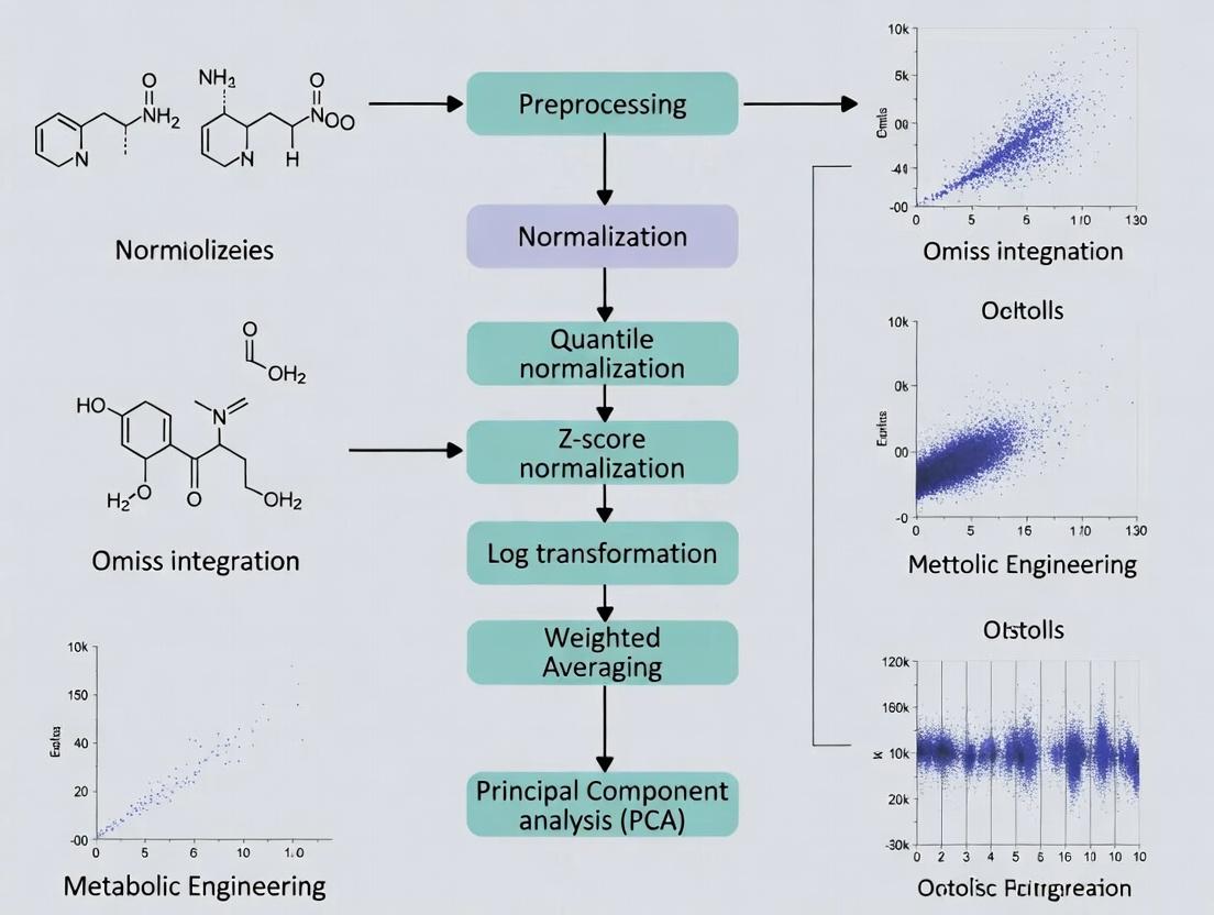
Diagram 1: Multi-Omic Data Integration Workflow

Diagram 2: Key Data Normalization Methods Taxonomy

Technical Support Center

Welcome to the technical support center for data normalization in omics integration research. This guide addresses common issues encountered during preprocessing of genomics, transcriptomics, and proteomics data.

Troubleshooting Guides & FAQs

• Q1: My principal component analysis (PCA) plot shows strong batch effects post-normalization. What went wrong?

  • A: This often indicates that the chosen normalization method is insufficient for the technical variation in your dataset. For multi-omics integration, consider:
    • Action: Apply a two-step normalization. First, use an intra-assay method (e.g., Quantile for RNA-seq). Second, employ a cross-platform method like ComBat or limma's removeBatchEffect to explicitly model and remove batch covariates.
    • Check: Verify your batch metadata is accurate and complete. Run a diagnostic like pvca (Principal Variance Component Analysis) to quantify the variance contributed by batch vs. biological factors.

• Q2: After log-transforming my proteomics data, I still have skewed distributions. How should I proceed?

  • A: Simple log transformation may not normalize data with heteroscedasticity (variance that changes with the mean).
    • Action: Implement Variance Stabilizing Normalization (VSN), which is designed for proteomics and microarray data. It simultaneously estimates a transformation and performs scaling to achieve homoscedasticity. Follow this protocol:
      • Load raw intensity data (from MaxQuant or DIA-NN) into R using the vsn package.
      • Apply the justvsn() function to the entire matrix.
      • Validate by plotting mean vs. standard deviation before and after transformation.

• Q3: I am integrating RNA-seq (counts) and microarray (intensities) data. Can I normalize them together?

  • A: No. Different technologies have distinct noise profiles and must be normalized separately before integration.
    • Action:
      • RNA-seq: Normalize using a method like DESeq2's median-of-ratios or edgeR's TMM on the count matrix.
      • Microarray: Normalize using limma's normalizeBetweenArrays (e.g., quantile normalization) on the log-intensity matrix.
      • Post-individual normalization: Use a cross-platform integration algorithm (e.g., MOFA+, DIABLO) that can handle residual technical differences, or perform an additional harmonization step like singular value decomposition (SVD) adjustment.

• Q4: How do I choose between Quantile Normalization and Median-centric scaling for my metabolomics dataset?

  • A: The choice depends on your assumption about the data.
    • Use Quantile Normalization if you assume the overall distribution of metabolite abundances should be identical across samples (e.g., in tightly controlled cell line studies). It forces all sample distributions to be the same.
    • Use Median-centric scaling (or Pareto scaling) if you expect only a subset of metabolites to change and wish to preserve more of the biological variance. This is common in clinical cohort studies. Median-centric divides each sample by its median intensity.

Quantitative Data Comparison of Common Normalization Methods

Table 1: Characteristics of Core Data Normalization Methods for Omics

Method	Primary Use Case	Assumption	Key Strength	Key Limitation
Quantile	Microarray, metabolomics	Overall distribution is consistent across samples.	Removes technical variation effectively; produces identical distributions.	Overly aggressive; can remove biological signal.
Median/IQR Scaling	Metabolomics, proteomics	Most features are not differentially abundant.	Simple, preserves structure of the data.	Less effective against severe batch effects.
TMM/Median-of-Ratios	RNA-seq (count data)	Most genes are not differentially expressed.	Robust to composition bias; good for heterogeneous samples.	Designed for count data only.
VSN	Proteomics, microarray	Technical variance is a function of mean intensity.	Stabilizes variance across the dynamic range.	More complex parameter estimation.
ComBat (Batch Correction)	All (post-initial norm.)	Batch effect is additive/multiplicative.	Powerful removal of known batch effects.	Risk of over-correction with small sample sizes.

Experimental Protocol: Two-Step Normalization for Multi-Batch RNA-seq Data

Title: Integrated Normalization and Batch Correction Protocol.

Objective: To generate comparable gene expression values from RNA-seq data derived from multiple sequencing runs or laboratories.

Materials:

• Raw gene count matrix (HTSeq-count, featureCounts output).
• Sample metadata file with Batch and Condition columns.
• R environment with DESeq2, sva, and limma packages installed.

Procedure:

• Primary Intra-Assay Normalization:
  • Create a DESeqDataSet object from the count matrix and metadata.
  • Estimate size factors using estimateSizeFactors. This performs median-of-ratios scaling.
  • Obtain normalized counts using counts(dds, normalized=TRUE). Log-transform (+1 pseudocount) for downstream analysis: log2(norm_counts + 1).

• Batch Effect Diagnosis:

  • Perform PCA on the log-transformed normalized matrix.
  • Color points by Batch and Condition. If samples cluster primarily by batch, proceed.

• Cross-Batch Harmonization (using limma):

  • Use the removeBatchEffect function: corrected_matrix <- removeBatchEffect(log_norm_matrix, batch=metadata$Batch, design=model.matrix(~Condition, data=metadata)).
  • Note: This function adjusts the data for batch effects while preserving the experimental design (Condition).

• Validation:

  • Re-run PCA on the corrected_matrix. Clusters should now be driven by Condition.

Visualization: Decision Workflow for Normalization

Title: Omics Data Normalization Decision Workflow

The Scientist's Toolkit: Research Reagent Solutions

Table 2: Essential Tools & Packages for Data Normalization Research

Item	Function	Example/Provider
R/Bioconductor	Open-source software environment for statistical computing and omics data analysis.	Core platform for all below packages.
limma	Fits linear models to assess differential expression for microarray/RNA-seq, includes removeBatchEffect.	Bioconductor Package.
DESeq2 / edgeR	Professional packages for normalization and differential analysis of RNA-seq count data.	Bioconductor Packages.
vsn	Performs variance stabilization and calibration for microarray or proteomics data.	Bioconductor Package.
sva	Contains ComBat and surrogate variable analysis for advanced batch effect modeling.	Bioconductor Package.
MOFA+	Bayesian framework for multi-omics integration, internally handles scale differences.	Python/R Package.
Reference Biomaterials	Standardized control samples (e.g., SCP, ERCC RNA spikes) to monitor technical variation.	Commercial vendors (e.g., Agilent, Thermo Fisher).

Technical Support Center: Troubleshooting Guides & FAQs

Frequently Asked Questions (FAQs)

Q1: My integrated multi-omics dataset shows strong batch effects after merging data from two sequencing runs. What are the first steps to diagnose and correct this? A1: The first step is to perform a Principal Component Analysis (PCA) or similar dimensionality reduction to visualize the data clustering by batch versus biological group. Use negative control samples or technical replicates if available. Apply a batch correction method such as ComBat, limma's removeBatchEffect, or Harmony, but only after ensuring batch is not confounded with your primary biological condition. Always validate correction by checking if batch-associated variance is reduced while biological signal is preserved.

Q2: How can I distinguish between a true biological confounder (e.g., patient age) and a technical artifact in my metabolomics data? A2: Conduct a variance partitioning analysis. Correlate the principal components (PCs) of your dataset with both technical (run date, instrument ID) and biological (age, BMI, sex) metadata. A technical artifact will typically correlate strongly with a single PC driven by batch, while a biological confounder will often spread across multiple PCs. Use linear mixed models (lmer in R) to quantify the proportion of variance explained by each factor.

Q3: My normalized RNA-seq counts show a systematic offset between samples processed with two different RNA extraction kits. Which normalization method is most robust? A3: When kit type is a known, recorded batch variable, consider using normalization methods that are robust to systematic shifts. For downstream differential expression, use methods like limma-voom with the batch factor included in the design matrix. For integration, Quantile Normalization or TMM (Trimmed Mean of M-values) followed by ComBat-seq can be effective. Avoid methods that assume all samples have the same global distribution if the batch effect is severe.

Q4: What quality control (QC) metrics are essential to monitor for technical variance in a high-throughput proteomics experiment? A4: Key QC metrics to track in a table format include:

• Total ion current (TIC) chromatogram consistency.
• Missing value rate per sample (should be <20% in label-free quant).
• Coefficient of variation (CV) for technical replicate pools across the run.
• Median coefficient of variation for all proteins across samples.
• Retention time drift over the experiment.

Q5: After applying a batch correction algorithm, how do I assess if I have over-corrected and removed biological signal? A5: Perform the following validation checks:

• Positive Controls: Check the signal strength of known, expected biological differences (e.g., treated vs. untreated controls) before and after correction. A significant drop is a red flag.
• Negative Controls: Check if biologically identical samples (replicates) still cluster together post-correction.
• Simulation: If possible, spike in synthetic biomarkers or use positive control genes/proteins to monitor their recovery.
• Downstream Analysis: Perform a pilot statistical test; the number of significant findings should be plausible, not zero or excessively high.

Troubleshooting Guides

Issue: High Technical Variance in Early Time Points in Cell-Based Screening Symptoms: Excessive variability in readouts (e.g., luminescence) for the first two columns of a 96-well plate compared to the rest. Diagnosis: This is often a "plate edge effect" or "equilibration effect" caused by temperature or CO₂ gradients while the plate stabilizes in the incubator. Solution:

• Protocol Adjustment: Begin the assay by seeding cells in the center wells first, moving outwards, or include a pre-incubation step where the filled plate rests in the incubator for 30 minutes before adding the stimulus.
• Experimental Design: Use randomized plate layouts for treatments and include dedicated negative/positive control wells distributed across the entire plate.
• Data Correction: Use spatial normalization within the plate, modeling the row and column effects using local regression (LOESS) on the control wells.

Issue: Drifting Baseline in LC-MS Metabolomics Runs Symptoms: Gradual increase or decrease in the total detected ion count or internal standard intensity over the sequence run time. Diagnosis: Instrument performance drift, often due to column degradation, source fouling, or changing mobile phase composition. Solution:

• Preventive Protocol: Implement a randomized sample injection order to avoid confounding drift with study group. Include blank washes and pooled QC samples every 4-6 injections.
• Corrective Data Processing: Use the QC samples for signal correction. Apply LOESS or smoothing spline regression to the QC feature intensities over run order, then use this model to adjust the experimental samples (e.g., using the stats::loess function in R).
• Reagent/Material: Use high-purity, mass-spec grade solvents and fresh mobile phases prepared daily.

Table 1: Common Normalization Methods for Multi-Omics Integration

Method Name	Primary Omics Use	Key Principle	Pros	Cons	Suitability for Integration
Quantile Normalization	Transcriptomics, Methylation	Forces all sample distributions to be identical.	Removes strong technical biases, makes distributions comparable.	Assumes most features are non-DE, can remove global biological variance.	Moderate. Use as initial step if platforms are identical.
TMM / RLE (DESeq2)	RNA-Seq	Estimates a sample-specific scaling factor relative to a reference.	Robust to a high proportion of differentially abundant features.	Designed for count data; less direct for other types.	Low for cross-omics. Can be used within RNA-seq data prior to integration.
ComBat / ComBat-seq	Multi-omics	Empirical Bayes framework to adjust for known batch effects.	Powerful for known batches, preserves within-batch variance.	Risk of over-correction; requires careful model specification.	High. Often used as a final step on individually normalized datasets.
Harmony / BBKNN	Single-cell, Multi-omics	Dimensionality reduction followed by iterative clustering and integration.	Integrates datasets without needing joint dimensionality reduction.	Computationally intensive; parameters need tuning.	Very High. State-of-the-art for integrating disparate datasets.
SVA / RUV-seq	Transcriptomics	Estimates surrogate variables for unmodeled technical factors.	Corrects for unknown confounders.	Can inadvertently remove biological signal; interpretation complex.	Moderate. Useful when batch factors are unrecorded.
Cyclic LOESS (MA)	Microarrays, Proteomics	Normalizes intensity-dependent biases by pairwise sample adjustment.	Non-parametric, performs well for two-color arrays.	Computationally slow for large datasets.	Low to Moderate. Mainly for within-platform normalization.
Median Polish / Robust Scaling	Metabolomics, Proteomics	Summarizes rows/columns by medians to calculate additive effects.	Simple, robust to outliers.	May not capture complex, non-additive biases.	Moderate. Simple baseline method for intensity data.

Experimental Protocols

Protocol 1: Performing a Batch Effect Diagnostic PCA Objective: To visualize and quantify the relative impact of batch versus biology on dataset variance. Materials: Normalized feature matrix (e.g., gene expression), metadata table with batch and group IDs, R/Python environment. Steps:

• Log-transform the normalized data if needed for variance stabilization.
• Center and scale the data (perform PCA on the correlation matrix).
• Compute principal components (PCs) using the prcomp() function in R or sklearn.decomposition.PCA in Python.
• Extract the variance explained by each PC.
• Correlate the sample coordinates (scores) for the top 10 PCs with both batch and biological group variables using linear models.
• Create a scatter plot of PC1 vs. PC2, colored by batch and shaped by biological group.
• Interpretation: If samples cluster primarily by batch in PC1/PC2, a significant batch effect is present. If biological groups separate well within batches, correction may be straightforward.

Protocol 2: Applying ComBat for Known Batch Correction Objective: To remove variation associated with a known batch factor (e.g., processing date) prior to integrative analysis. Materials: Feature matrix (one omics type), batch variable, optional biological covariates. Software: R package sva. Steps:

• Data Preparation: Ensure your input data (dat) is a normalized matrix (features x samples). Define your batch variable (batch) and a model matrix for any biological covariates you wish to preserve (mod).

• Run ComBat: Use the ComBat function for normally distributed data (e.g., microarray, log-transformed RNA-seq).

• Validation: Repeat the diagnostic PCA (Protocol 1) on the corrected_data. The correlation between top PCs and the batch variable should be minimized.

Visualizations

Title: Multi-Omics Integration & Batch Correction Workflow

Title: Decision Tree for Confounder and Batch Effect Management

The Scientist's Toolkit: Research Reagent Solutions

Table 2: Essential Reagents & Materials for Mitigating Technical Variance

Item	Function in Mitigating Variance	Example Product/Kit	Key Consideration
Universal Reference RNA	Provides an inter-laboratory, inter-platform standard for transcriptomics to calibrate and benchmark performance.	Stratagene Universal Human Reference RNA, ERCC ExFold RNA Spike-In Mix	Use at consistent dilution across all batches to track technical sensitivity.
Pooled QC Samples	A homogenized aliquot of sample material run repeatedly throughout the sequence to monitor and correct for instrument drift.	Custom-made pool from a subset of study samples.	Must be representative of the entire sample set (e.g., mix equal amounts from all groups).
Internal Standards (IS)	Corrects for variability in sample prep, injection volume, and ion suppression in MS-based proteomics/metabolomics.	Stable Isotope-Labeled peptides (AQUA), Deuterated metabolites.	Should be added as early as possible in the protocol and cover a range of chemical properties.
Blocking/Matched Reagents	Minimizes non-specific binding and variability in immunoassays (ELISA, Luminex).	Blocking Buffers (BSA, Casein), Antibody Diluents.	Must be optimized for the specific antibody-antigen pair to reduce background noise.
DNA/RNA Storage Stabilization Buffer	Preserves nucleic acid integrity at variable temperatures pre-processing, reducing degradation-related bias.	RNA_later, DNA/RNA Shield.	Crucial for multi-center studies with inconsistent cold chain logistics.
Single-Lot Assay Kits/Plates	Using the same manufacturing lot for a large study reduces kit-to-kit reagent variability.	All ELISA, qPCR Master Mix, or sequencing library prep kits from the same lot.	Requires advanced planning and procurement for large-scale studies.
Automated Liquid Handlers	Improves precision and reproducibility of pipetting steps compared to manual handling, especially for high-throughput screens.	Beckman Coulter Biomek, Hamilton STAR, Echo Acoustic Liquid Handler.	Requires regular calibration and validation of dispensed volumes.

Technical Support Center: Troubleshooting Guides & FAQs

FAQ 1: Why does my integrated multi-omics analysis show high technical batch effects even after quantile normalization? Answer: Quantile normalization assumes all samples have identical distribution, which is often violated in multi-batch omics studies. This method fails to correct for non-linear batch-specific biases. Implement a two-step correction: First, use ComBat or limma::removeBatchEffect on each omics dataset separately. Then, apply a cross-platform normalization like SVA or RUVseq on the integrated matrix. Always validate with PCA plots pre- and post-correction, using batch as a color variable.

FAQ 2: How do I handle missing values in proteomics data before integrating with transcriptomics? Answer: The strategy depends on the nature of the 'missingness'. For data missing not at random (MNAR), typical in proteomics, use methods tailored to left-censored data.

• For low % missing (<10%): Impute with knn or Random Forest (see Protocol 1).
• For high % missing (>20%): Use a multi-step approach: 1) Filter proteins with >50% missingness. 2) For remaining, apply QRILC (Quantile Regression Imputation of Left-Censored data) or MinProb imputation. 3) Validate imputation by checking the distribution of complete and imputed values.

FAQ 3: My pathway analysis results differ drastically between single-omics and integrated multi-omics approaches. Which should I trust? Answer: Discrepancies are expected. Single-omics analysis identifies pathways dysregulated at one molecular layer. Integrated analysis (e.g., multi-optic factor analysis) reveals convergent pathways across layers, often more biologically coherent. Trust the integrated result if your normalization pipeline is sound (see Protocol 2). Use a consensus score (e.g., integrative pathway enrichment via IMPaLA or multiGSEA) to rank pathways by combined evidence.

FAQ 4: What is the best method to normalize scRNA-seq data for integration with bulk proteomics? Answer: Direct integration is challenging due to sparsity and scale differences. Recommended workflow:

• Normalize scRNA-seq: Use SCTransform (v2 regularized negative binomial) to stabilize variances and remove technical noise.
• Pseudobulk Creation: Aggregate scRNA-seq counts by sample/condition to create a "bulk-like" expression profile.
• Cross-platform scaling: Apply a mutual information-based scaling method (e.g., MMD-MA or Seurat's CCA anchor-based integration for paired samples) to align the two feature spaces.
• Validation: Correlate key ligand-receptor pair expression between platforms.

---

Experimental Protocols

Protocol 1: Random Forest Imputation for Missing Proteomics Values

Objective: Accurately impute missing values (MNAR) in a protein intensity matrix. Materials: See "Research Reagent Solutions" table. Method:

• Pre-processing: Log2-transform the complete portion of your intensity matrix.
• Initialization: Impute all missing values using the minimum value per column (protein) shifted down by a small noise distribution (mean=0, sd=0.1).
• Iterative Imputation: Use the missForest R package (or sklearn.ensemble.IterativeImputer in Python).
  • Set maxiter = 10, ntree = 100.
  • For each iteration, the random forest predicts missing values for each protein using all other proteins as predictors.
  • Stop when the imputed matrix difference between iterations is below a set threshold (tolerance = 0.01).
• Post-imputation: Reverse the log2 transformation to return to a linear scale for downstream integration.

Protocol 2: Multi-Omic Data Integration via MOFA+

Objective: Integrate normalized matrices from transcriptomics, proteomics, and metabolomics to identify latent factors driving variation. Method:

• Input Preparation: Ensure each omics data view is a samples x features matrix, independently normalized and scaled (e.g., Z-scored across features).
• Model Training: Run MOFA+ (v1.0+).

• Factor Interpretation: Use plot_factor_cor(mofa_trained) to check for technical factor associations and plot_weights(mofa_trained, view="transcriptomics") to identify top feature loadings.
• Downstream Analysis: Regress factor values against clinical phenotypes to identify biologically relevant latent drivers.

---

Data Presentation

Table 1: Comparison of Normalization Methods for Bulk RNA-seq Integration

Method	Principle	Best For	Key Metric (Median CV Reduction)	Suitability for Cross-Omics
DESeq2 (Median of Ratios)	Size factor based on geometric mean	Within-platform RNA-seq	25-30%	Low
TMM (edgeR)	Trimmed Mean of M-values	RNA-seq with composition bias	28-33%	Medium
Cross-Contaminant Correction (CCC)	Mutual information maximization	RNA-seq + Proteomics	40-45%*	High
Quantile Normalization	Empirical distribution alignment	Microarray platforms	20-25%	Medium
Cyclic LOESS (limma)	Intensity-dependent smoothing	Multi-batch microarray	35-40%	Medium

Data synthesized from recent benchmarks (Smyth et al., 2023; Prakash et al., 2024). CV = Coefficient of Variation.

---

Diagrams

Diagram 1: Multi-Omic Integration Workflow

Diagram 2: Missing Data Imputation Decision Tree

---

The Scientist's Toolkit: Research Reagent Solutions

Table 2: Essential Reagents & Tools for Normalized Integration Experiments

Item	Function in Integration Pipeline	Example Product/Code
Reference RNA Sample	Inter-batch calibration standard for transcriptomics.	Universal Human Reference RNA (Agilent)
Pooled QC Sample	A consistent sample injected in each batch to track and correct LC-MS/MS (proteomics/metabolomics) performance drift.	Pooled from equal aliquots of all study samples
Isotope-Labeled Internal Standards	Absolute quantification and normalization in mass spectrometry-based assays.	Thermo Scientific Pierce Heavy Peptide Standards
Batch Effect Correction Software	Statistical removal of technical variation.	sva R package (ComBat), limma
Multi-Omic Integration Suite	Joint dimensionality reduction and factor analysis.	MOFA+ (R/Python), mixOmics
Containerization Software	Ensures computational reproducibility of the entire pipeline.	Docker, Singularity

A Practical Toolkit: Key Data Normalization Methods for Each Omics Layer

Troubleshooting Guides & FAQs

Q1: After applying within-sample normalization (e.g., using housekeeping genes), my across-sample batch effects appear worse. What went wrong? A: This is a common pitfall. Within-sample normalization controls for technical variation within a single run (e.g., differences in total RNA input). It is not designed to correct for systematic technical variation between different batches or experimental runs. Applying within-sample methods first can sometimes amplify across-sample differences. The recommended workflow is to:

• Perform within-sample normalization.
• Integrate or batch-correct your data using dedicated across-sample methods (e.g., ComBat, limma's removeBatchEffect, or integration tools like Harmony).
• Always visualize data with PCA before and after each step to assess the impact.

Q2: For single-cell RNA-seq, should I perform normalization within each cell or across the entire cell population? A: You typically need both, in sequence. First, normalize within each cell to account for differences in sequencing depth (e.g., using "Total Count" or "DESeq2's median-of-ratios" normalization per cell). This gives you comparable expression values across cells. Second, you must scale the data across cells to center and variance-stabilize the expression of each gene, enabling dimensionality reduction and clustering. This two-step process is standard in pipelines like Seurat (NormalizeData followed by ScaleData).

Q3: When integrating proteomics data from different platforms (e.g., label-free and TMT), which normalization scope is primary? A: Across-sample (cross-platform) normalization is critical. First, perform within-run normalization for each platform separately (e.g., median centering for label-free). Then, you must apply a robust across-sample method to align the distributions from different platforms. Methods like Quantile Normalization or robust scaling (e.g., using "reference" samples run on both platforms) are often employed. Failure to do this will result in platform-driven clustering.

Q4: My normalized data shows high correlation between technical replicates but poor correlation between biological replicates. Is this a normalization issue? A: Not necessarily. Strong technical replicate correlation validates that your within-sample normalization is working correctly to minimize run-to-run noise. Poor biological replicate correlation suggests high biological variability or potential issues in experimental design/sample collection. Normalization cannot create biological consistency; it can only remove technical bias. Investigate sample quality and biological variance sources.

Q5: Does log-transformation count as within-sample or across-sample normalization? A: Log-transformation (e.g., log2(x+1)) is a variance-stabilizing transformation, not a normalization step per se. However, it is applied across all samples universally to make the data conform to statistical modeling assumptions (homoscedasticity). It is typically applied after within-sample count normalization but before across-sample batch correction.

Experimental Protocols

Protocol 1: Two-Step Normalization for Bulk RNA-Seq Integration Objective: Integrate RNA-seq datasets from two studies performed at different sequencing centers.

• Within-Sample Normalization:
  • Input: Raw gene count matrices from each study.
  • Method: Apply DESeq2's "median of ratios" method separately to each dataset. This corrects for library size and RNA composition bias within each study.
  • Output: Normalized count matrices.
• Across-Sample Normalization & Batch Correction:
  • Input: Combined normalized count matrices from step 1.
  • Method: Use the sva package's ComBat function, treating "Study" as the known batch covariate. Optional: include biological covariates (e.g., disease status) in the model to preserve.
  • Validation: Perform PCA. Batch clustering (by study) should be minimized, while biological group clustering should be maintained or enhanced.

Protocol 2: Normalization for Cross-Platform Metabolomics Objective: Align peak intensity data from GC-MS and LC-MS runs.

• Within-Sample (Within-Run) Normalization:
  • For each run, calculate the median intensity of all peaks or of a set of stable internal standards.
  • Divide all peak intensities in that run by this median value.
  • This sets the median intensity to 1 for each run, controlling for overall signal strength differences.
• Across-Sample (Between-Platform) Alignment:
  • Identify a set of metabolites confidently detected in both platforms.
  • For these "bridge" metabolites, calculate a scaling factor based on the ratio of their median intensities (LC-MS/GC-MS) across all shared samples.
  • Apply this platform-specific scaling factor to all metabolites from the respective platform before merging datasets.

Table 1: Common Normalization Methods by Scope

Scope	Method Name	Primary Use Case	Key Assumption
Within-Sample	Total Count / Library Size	Bulk RNA-seq, early single-cell RNA-seq	Total read output per sample is representative of input.
Within-Sample	DESeq2's Median of Ratios	Bulk RNA-seq	Most genes are not differentially expressed.
Within-Sample	TMM (Trimmed Mean of M-values)	Bulk RNA-seq between experiments	The majority of genes are non-DE and expression is symmetric.
Across-Sample	Quantile Normalization	Microarrays, making distributions identical	The empirical distribution across samples should be the same.
Across-Sample	ComBat / limma removeBatchEffect	Removing known batch effects	Batch effects are additive or multiplicative and can be modeled.
Across-Sample	Z-score / Standard Scaling	Proteomics, metabolomics, pre-ML	Features should have mean=0 and SD=1 across samples.

Table 2: Impact of Normalization Scope on Data Metrics

Analysis Metric	Before Any Normalization	After Within-Sample Only	After Within & Across-Sample
Correlation (Technical Replicates)	Low (e.g., 0.85-0.92)	High (e.g., >0.98)	Maintains High
PCA Plot: Batch Clustering	Strong	May Persist or Change	Minimized
PCA Plot: Biological Group Separation	Obscured by Batch	May Improve	Optimal
Differential Expression False Positives	Very High	Reduced	Minimized

Visualizations

Title: Sequential Normalization Workflow for Data Integration

Title: Methods Categorized by Within vs. Across-Sample Scope

The Scientist's Toolkit: Research Reagent Solutions

Item / Reagent	Function in Normalization Context
Spike-in RNAs (e.g., ERCC)	Exogenous controls added at known concentrations for across-sample normalization, especially in single-cell RNA-seq, to distinguish technical noise from biological variation.
Housekeeping Gene Panels	Endogenous genes assumed to have stable expression across samples/conditions. Used as internal reference for within-sample normalization in qPCR and some sequencing analyses.
Internal Standards (IS) - Isotopically Labeled	Chemically identical but heavy-isotope-labeled compounds spiked into each sample in proteomics/metabolomics. Corrects for within-sample ionization efficiency and across-sample instrument drift.
Reference/QC Pool Sample	A homogeneous sample (mix of all study samples) run repeatedly across batches/platforms. Serves as a technical anchor for across-sample alignment and monitoring of longitudinal performance.
UMI (Unique Molecular Identifier)	Short random barcodes attached to each mRNA molecule before amplification in single-cell protocols. Enables within-sample correction for PCR amplification bias by deduplication.
Bead-Based Counting (e.g., 10x Genomics)	Provides an accurate estimate of the number of recovered cells, forming the basis for within-sample "cell-aware" normalization in single-cell genomics.

Troubleshooting Guides & FAQs

Q1: My quantile-normalized gene expression matrix shows reduced biological variance between sample groups. What went wrong? A: This is a known risk when applying quantile normalization to datasets with assumed global differences. The method forces the distribution of all samples to be identical, which can remove true biological signal. Solution: Use diagnostic plots pre- and post-normalization. Compare the distributions of sample groups using boxplots. If groups were globally different (e.g., case vs. control had systematically higher expression), quantile normalization is inappropriate. Consider using a method like TMM (for RNA-seq) that assumes only a subset of genes are differential.

Q2: After Median/IQR scaling, my proteomics data still has batch effects. Why wasn't it removed? A: Median/IQR scaling (often a form of robust z-scoring) is primarily a within-sample normalization. It centers and scales each sample's measurements but does not align distributions across samples or batches. Solution: Apply Median/IQR scaling per sample first to handle technical variance within runs. Then, apply a between-sample batch correction method (e.g., ComBat, limma's removeBatchEffect) using your batch metadata. The workflow should be: 1) Within-sample scaling, 2) Between-sample batch correction.

Q3: When calculating Z-scores for metabolomics integration, should I scale by feature (metabolite) or by sample? A: This is context-critical and a common source of error. Scaling by sample (column) is used to make samples comparable, often after an initial normalization. Scaling by feature (row) is used to identify which metabolites are most elevated/depleted in a given sample. For integration, the goal is typically to make samples comparable. Solution: For multi-omics integration where samples are the common unit, scale by feature (metabolite/gene) across all samples. This places all measurements on a common, unit-less scale (mean=0, sd=1) for each analyte, enabling cross-dataset comparison.

Q4: TMM normalization fails with an error about zero library sizes or all-zero counts for some samples in my single-cell RNA-seq project. A: TMM calculates scaling factors relative to a reference sample, and zero or extremely low library sizes can break its log-ratio calculations. Solution:

• Pre-filtering: Remove genes with zero counts across all cells and filter out cells (samples) with an extremely low total count (library size) prior to TMM. This is often done in quality control.
• Pseudo-count: While TMM uses a log transformation inherently, ensure your count matrix hasn't been improperly transformed prior to TMM input. TMM should be run on raw counts.
• Alternative: For sparse single-cell data, consider alternate normalization-scaling methods like those in Seurat (log normalization) or SCTransform.

Q5: For integrating microarray and RNA-seq data, which normalization method is most robust? A: Direct application of any single method (Quantile, Z-score, etc.) to the combined raw data will fail due to platform-specific technical distributions. Solution: A two-stage approach is required:

• Within-platform normalization: Normalize each dataset separately using platform-appropriate methods (e.g., Quantile for microarray, TMM for RNA-seq).
• Between-platform alignment: Use a cross-platform normalization method, such as ComBat (for known batch=platform) or Cross-Platform Normalization (XPN), on the combined, separately normalized data. This aligns the statistical distributions without removing biological signal.

Table 1: Comparison of Core Normalization Techniques

Technique	Primary Use Case	Assumptions	Robust to Outliers?	Output Data Scale
Quantile	Microarray data, making sample distributions identical.	The overall distribution of expression is similar across samples.	No	All samples have identical value distribution.
Median/IQR	Scaling individual samples (e.g., metabolomics, proteomics runs).	The median and spread of the sample is a good technical reference.	Yes (uses median, not mean)	Each sample median=0, IQR=1.
Z-Score	Placing features (genes/metabolites) on a comparable scale for integration.	Data is roughly normally distributed per feature.	No (uses mean, SD)	Each feature has mean=0, standard deviation=1 across samples.
TMM	RNA-seq data (bulk) to correct for library size and composition.	Most genes are not differentially expressed (DE), and DE is symmetric.	Yes (uses trimmed mean)	Effective library size adjusted, log-CPM values are comparable.

Table 2: Suitability for Omics Data Types

Data Type	Recommended Primary Normalization	Key Consideration
RNA-seq (Bulk)	TMM (or related: DESeq2's median-of-ratios)	Addresses composition bias and varying sequencing depths.
Microarray	Quantile Normalization	Standard for Affymetrix/Illumina to force identical distributions.
Proteomics (Label-Free)	Median/IQR per sample, then between-sample alignment.	High technical variance per run; median is robust to high-abundance outliers.
Metabolomics	Sample-specific scaling (Median/IQR), followed by feature-wise Z-scoring for integration.	Handles run drift and puts diverse metabolites on a common scale.
Multi-Omics Integration	Platform-specific method first, then feature-wise Z-scoring across the combined dataset.	Harmonizes vastly different numerical ranges and variances from each platform.

Experimental Protocols

Protocol 1: Executing TMM Normalization for Bulk RNA-seq Data (via edgeR)

• Input: Raw count matrix (genes x samples).
• Filtering: Remove genes with very low counts (e.g., filterByExpr in edgeR).
• DGEList Object: Create a DGEList object containing the counts and sample group information.
• Calculate Factors: calcNormFactors(object, method = "TMM") computes scaling factors for each sample relative to a reference sample (geometric mean of all libraries).
• Output: The DGEList object now contains the $samples$norm.factors. These factors are used in downstream differential expression models to offset library sizes.

Protocol 2: Cross-Platform Integration of Microarray and RNA-seq Data

• Separate Normalization:
  • Microarray Data: Apply Quantile Normalization (e.g., normalize.quantiles() from preprocessCore package).
  • RNA-seq Data: Apply TMM normalization and convert to log2-Counts-Per-Million (log2-CPM) using the cpm() function in edgeR with prior count.
• Common Gene Space: Map both datasets to a common gene identifier (e.g., official gene symbol) and retain only intersecting genes.
• Batch Correction: Treat "platform" as a batch covariate. Use the ComBat function from the sva package on the combined, log-transformed matrices ([Microarray, RNA-seq]). Specify the platform as the batch parameter.
• Validation: Perform PCA on the integrated matrix. Samples should cluster by biological group, not by platform (batch).

Visualizations

Multi-Omics Integration Workflow

TMM Normalization Process for RNA-seq

The Scientist's Toolkit: Research Reagent Solutions

Item / Resource	Function in Normalization & Integration
edgeR / limma (R packages)	Industry-standard tools for TMM normalization and differential expression analysis of RNA-seq and microarray data.
preprocessCore (R package)	Provides optimized, efficient algorithms for quantile normalization of large datasets (microarrays).
sva / ComBat (R packages)	Critical for removing batch effects (technical, platform, lab) in high-dimensional data prior to integration.
Reference RNA Samples (e.g., ERCC Spike-Ins)	Synthetic exogenous controls added to RNA-seq experiments to monitor technical variance and sometimes aid normalization.
Common Gene ID Mappers (e.g., biomaRt, EnsDb)	Essential for mapping gene identifiers across platforms (e.g., Ensembl ID to Symbol) to find the common feature space for integration.
RobustScaler / StandardScaler (Python, scikit-learn)	Implementations of Median/IQR (robust) and Z-score (standard) scaling for Python-based analysis pipelines.
Single-Cell Specific Tools (e.g., Seurat, Scanpy)	Provide tailored normalization methods (e.g., log-normalization, SCTransform) for sparse single-cell data where TMM may fail.

Technical Support Center

Troubleshooting Guides & FAQs

Q1: My ComBat-corrected data still shows strong batch separation in the PCA. What went wrong? A: This often indicates that the batch variable is confounded with a biological variable of interest (e.g., all controls from Batch 1, all treatments from Batch 2). ComBat cannot disentangle these. First, visually inspect the design.

• Actionable Protocol: Create a design matrix modeling your biological factor. Use model.matrix(~biological_group, data=pheno_data). Then, run ComBat with the mod parameter set to this matrix: ComBat(dat=expression_matrix, batch=batch_vector, mod=design_matrix). This protects the biological signal while removing batch effects orthogonal to it.

Q2: When using SVA, how do I determine the correct number of surrogate variables (SVs) to estimate? A: Over-estimation removes biological signal; under-estimation leaves residual batch effects.

• Actionable Protocol: Use the num.sv function from the sva package with a null and full model. The recommended method is based on asymptotic BIC.

Q3: After using removeBatchEffect, my corrected data yields perfect group separation. Is this valid for downstream differential expression? A: No. This is a critical misuse. limma::removeBatchEffect is designed for visualization, not for direct input into differential expression (DE) tests. It removes batch-associated variation without preserving the statistical uncertainty needed for DE.

• Actionable Protocol: For correct DE analysis with batch correction, incorporate the batch term directly into your linear model in limma.

Q4: I get an error "Error in solve.default(t(mod) %*% mod) : system is computationally singular" in ComBat. How do I fix it? A: This indicates perfect collinearity in your model matrix (mod). Your model is over-specified (e.g., including a covariate that is a linear combination of batch).

• Actionable Protocol: Check the rank of your design matrix: qr(design_matrix)$rank. It must be less than the number of columns. Simplify the model by removing the confounded covariate. If biological group and batch are perfectly confounded, batch correction is statistically impossible without additional prior information.

Q5: Should I correct for batch effects before or after normalizing my RNA-seq/gene expression data? A: Batch correction is typically the final step in pre-processing, applied to already normalized (e.g., TPM, FPKM, or log2-counts-per-million) and filtered data.

• Standardized Workflow Protocol:
  • Raw Counts: Start with a counts matrix.
  • Filtering: Remove lowly expressed genes (e.g., requiring >10 counts in at least n samples).
  • Primary Normalization: Apply between-sample normalization for library size and composition (e.g., TMM normalization in edgeR, or variance stabilizing transformation in DESeq2).
  • Transformation: Log2-transform the normalized data (e.g., log2(CPM + k)).
  • Batch Correction: Apply ComBat, SVA, or removeBatchEffect to the log2-transformed, normalized data.

Table 1: Key Characteristics of Batch Correction Methods

Feature	ComBat (sva package)	Surrogate Variable Analysis (SVA)	limma::removeBatchEffect
Core Approach	Empirical Bayes shrinkage of batch means.	Estimates hidden factors (SVs) from data residuals.	Simple linear model to subtract batch means.
Model Flexibility	High. Can include biological covariates (mod).	High. Models biological factors to protect signal.	Moderate. Can include other covariates.
Preserves DE Integrity	Yes, when used correctly with mod.	Yes, SVs are added to the DE model.	No. For visualization only.
Handles Unknown Factors	No. Only known batches.	Yes. Primary strength is estimating unknown SVs.	No. Only known batches.
Output Data Use	Direct input for DE/analysis (with caution).	SVs used as covariates in DE model; corrected data for visualization.	Visualization and clustering only.
Best For	Adjusting for known, documented batch effects.	Complex studies with unmeasured confounders.	Preparing publication-quality plots.

The Scientist's Toolkit: Research Reagent Solutions

Table 2: Essential Tools for Batch Effect Correction & Analysis

Item	Function & Relevance
R/Bioconductor	The essential software environment for statistical analysis of omics data.
sva Package	Contains the ComBat and sva functions for empirical Bayes correction and surrogate variable estimation.
limma Package	Industry-standard package for linear modeling of omics data, includes removeBatchEffect.
High-Quality Phenotypic Metadata	Accurate, detailed sample information (batch, processing date, technician, biological group) is the most critical non-software "reagent."
Reference RNA Samples	Technical controls (e.g., Universal Human Reference RNA) spiked-in across batches to diagnose and quantify batch effects.
ggplot2 & pheatmap Packages	For creating PCA plots and heatmaps pre- and post-correction to visually assess effectiveness.

Methodology & Visualization

Experimental Protocol: Integrated Batch Correction Assessment

• Data Preparation: Log2-transform your normalized expression matrix. Generate a PCA plot (colored by batch and biological group) as a baseline.
• Correction Execution:
  • ComBat: Execute combat_corrected <- ComBat(dat=log2_data, batch=batch, mod=model.matrix(~group)). Store output.
  • SVA: Estimate SVs using the protocol in Q2. Correct data using cleanY function or by regressing out SVs: corrected <- lmFit(log2_data, model.matrix(~group + svobj$sv))$residuals + matrix(apply(log2_data, 1, mean), ncol=ncol(log2_data), nrow=nrow(log2_data)).
  • removeBatchEffect: Execute limma_corrected <- removeBatchEffect(log2_data, batch=batch, design=model.matrix(~group)).
• Assessment: Generate PCA plots for each corrected dataset. Calculate key metrics: (a) Percent of variance explained by batch before/after (PERMANOVA), and (b) Average within-biological-group variance.

Diagram: Batch Correction Decision Workflow

Title: Choosing a Batch Correction Method

Diagram: Omics Data Pre-processing Pipeline

Title: Standard Omics Pre-processing Workflow

Technical Support Center: Troubleshooting Guides & FAQs

This support center provides solutions for common issues encountered when applying RPKM, TPM, LFQ, and PQN normalization within integrated omics studies, a core component of robust data integration for multi-omics research.

FAQs & Troubleshooting

Q1: My RPKM values from RNA-seq are highly correlated with gene length. Is this normal, and how does it affect integration with proteomics (LFQ) data? A: Yes, RPKM (Reads Per Kilobase per Million mapped reads) inherently retains a length bias. This can confound integration with LFQ proteomics data, where quantification is less directly length-dependent.

• Troubleshooting: Use TPM (Transcripts Per Million) instead. TPM reverses the order of operations, normalizing for gene length first, which mitigates this bias and yields more comparable distributions for integration.

Q2: After LFQ normalization in MaxQuant, my proteomics data still shows a batch effect across experimental runs. What should I do? A: MaxQuant's LFQ algorithm normalizes for run-to-run variation, but strong batch effects may persist.

• Troubleshooting: Apply an additional post-processing normalization like PQN (Probabilistic Quotient Normalization). Use the median spectrum from all high-quality samples as a reference to correct for systematic shifts. Ensure batch information is included in your experimental design for statistical modeling later.

Q3: When applying PQN to my metabolomics dataset, some features become disproportionately scaled. What could be the cause? A: This often occurs when the chosen reference spectrum (e.g., median sample) is not representative of the entire dataset, or if the dataset contains many missing values or non-biological outliers.

• Troubleshooting:
  • Pre-filter: Remove features with >20% missing values and impute the remainder (e.g., with k-nearest neighbors).
  • Reference Selection: Visually inspect PCA plots to identify a representative sample pool. Consider using a pooled QC sample as the reference if available.
  • Iterate: Recalculate the median reference after removing obvious outlier samples.

Q4: How do I handle zero or missing values when calculating TPM or applying PQN? A: These methods handle zeros differently.

• TPM: Zero counts are valid and remain zero. Do not impute before TPM calculation.
• PQN: Zeros/missing values are problematic. Imputation (e.g., with half the minimum positive value for the feature) is required before PQN to calculate reliable quotients. Always document your imputation strategy.

Q5: Can I directly compare TPM (transcriptomics) and LFQ intensity (proteomics) values after normalization? A: No. While each method renders data within its platform comparable, the absolute scales between platforms are different.

• Troubleshooting: For integration, further steps are needed: 1) Within-platform standardization (e.g., z-scoring), or 2) Model-based integration (e.g., multi-omics factor analysis) which operates on relative patterns, not raw normalized values.

Key Experimental Protocols

Protocol 1: Generating TPM from RNA-seq Read Counts

• Input: Gene/transcript raw count matrix (post-alignment and quantification with tools like HTSeq or featureCounts).
• Calculate Reads per Kilobase (RPK): Divide the read counts for each gene by its length in kilobases. RPK = Count / (Gene Length / 1000)
• Calculate Per Million Scaling Factor: Sum all RPK values in a sample and divide by 1,000,000.
• Calculate TPM: Divide each gene's RPK value by the sample-specific scaling factor. TPM = RPK / Scaling Factor
• Output: A matrix where the sum of all TPM values in each sample is 1,000,000.

Protocol 2: LFQ Normalization in MaxQuant (Typical Workflow)

• Raw Data Input: Provide Thermo .raw files and a experimental design template.
• Parameter Setting: In the Group-specific parameters tab, check the "LFQ" box. Set the LFQ min. ratio count to 2 (default). Match retention times between runs.
• Processing: MaxQuant performs:
  • Feature detection and MS/MS identification.
  • Intensity extraction for all features across all runs.
  • LFQ Algorithm: Pairs MS1 feature intensities between runs, constructs an intensity profile matrix, and normalizes using a stable median ratio between runs.
• Output: The proteinGroups.txt file with columns LFQ intensity_[Sample] for downstream analysis.

Protocol 3: Applying PQN to Metabolomics/Proteomics Data

• Input: A feature intensity matrix (samples x features), post-missing value imputation.
• Calculate the Reference: Typically, the median spectrum (feature-wise median across all samples) is computed.
• Calculate Quotients: For each sample, divide the intensity of each feature by the corresponding intensity in the reference spectrum.
• Determine the Scaling Factor: Calculate the median of all quotients for that sample.
• Normalize: Divide all feature intensities in the sample by its median scaling factor.
• Output: A matrix corrected for global dilution/concentration differences, preserving biological variance ratios.

Table 1: Comparison of Normalization Methods Across Omics Domains

Method	Primary Domain	Core Purpose	Handles Zeros?	Removes Sample Dilution Effect?	Output Scale
RPKM/FPKM	Transcriptomics	Enables comparison of expression levels across genes and samples.	Yes (zeros remain).	No	Not sum-constrained
TPM	Transcriptomics	Improved within-sample comparison; mitigates gene length bias.	Yes (zeros remain).	No	Sum = 1 million per sample
LFQ (MaxQuant)	Proteomics	Label-free quantification correcting run-to-run variation.	Yes (inferred from matched runs).	Partially (via median ratios)	Log2 transformed intensities
PQN	Metabolomics/Proteomics	Corrects for global concentration/dilution differences (e.g., urine).	No (requires imputation).	Yes	Preserves original unit ratios

Visualizations

Title: TPM Calculation Workflow from Raw Counts

Title: Probabilistic Quotient Normalization (PQN) Logic

Title: Normalization Path for Multi-Omics Integration

The Scientist's Toolkit: Research Reagent & Essential Materials

Table 2: Essential Resources for Omics Normalization Experiments

Item	Function in Context	Example/Note
High-Quality Reference Genome/Proteome	Essential for accurate read/gene assignment (RPKM/TPM) and peptide identification (LFQ).	Ensembl, RefSeq, UniProt. Version control is critical.
Spike-in Controls (External)	Added to samples prior to processing to monitor technical variation for potential post-LFQ/PQN correction.	S. pombe spike-in for RNA-seq; stable isotope-labeled peptide/protein standards for proteomics.
Pooled Quality Control (QC) Sample	A mixture of all study samples, run repeatedly throughout the MS sequence. Serves as a robust reference for PQN and monitors instrument stability for LFQ.	Crucial for metabolomics and proteomics batch correction.
Standard Reference Material	Provides a known benchmark to assess quantification accuracy across platforms.	NIST SRM 1950 (metabolites in plasma), UPS2 proteome standard.
Bioinformatics Software/Packages	Implement the normalization algorithms and downstream integration.	RSEM/Kallisto for TPM; MaxQuant for LFQ; R/Python (e.g., nortools package) for PQN; MOFA2, mixOmics for integration.
Parameter Configuration File	A documented text file specifying all software settings (e.g., MaxQuant mqpar.xml). Ensures reproducibility of LFQ/TPM results.	Must be archived with the raw data.

Technical Support Center

Troubleshooting Guides & FAQs

Q1: I receive "Error in svd(x, nu = 0) : infinite or missing values in 'x'" when running ComBat from the sva package in R. What does this mean and how do I fix it?

A: This error indicates your input data matrix contains NA, NaN, or infinite values, which the SVD calculation cannot process. To resolve:

• Check for NAs: Run sum(is.na(your_data_matrix)) or any(is.infinite(your_data_matrix)).
• Filter or Impute: Remove features (rows) with excessive missing values or use imputation. For gene expression, consider impute.knn from the impute package.
• Protocol: Before running ComBat, clean your data:

Q2: When using sklearn.preprocessing.StandardScaler for single-cell RNA-seq data normalization, my downstream clustering results are poor. Am I applying it incorrectly?

A: Likely yes. StandardScaler scales features (genes) to mean=0 and variance=1, which can amplify technical noise in sparse scRNA-seq data. This method is not typical for primary count normalization.

• Correct Workflow: Apply gene- or sample-specific scaling after count normalization and transformation.
• Protocol:

Q3: How do I choose between removeBatchEffect (limma) and ComBat (sva) for correcting batch effects in my multi-omic dataset integration?

A: The choice depends on study design and data structure. See the comparison table below.

Table 1: Comparison of Common Batch Effect Correction Methods in R

Method (Package)	Primary Use Case	Key Assumption	Handles Complex Design?	Output For
removeBatchEffect (limma)	Linear models, microarray/RNA-seq	Batch effects are additive	Yes (uses design matrix)	Downstream linear modeling (e.g., DE analysis)
ComBat / ComBat_seq (sva)	Empirical Bayes, high-dimensional data	Batch means and variances follow a prior distribution	Limited (uses model with intercept)	Exploratory analysis & clustering
fastMNN (batchelor)	scRNA-seq integration, mutual nearest neighbors	A subset of cells are biological matches across batches	Yes	Common low-dimensional embedding for clustering

Q4: I get convergence warnings when running ComBat with many batches (>20). Is the result still reliable?

A: Warnings may occur with many small batches. Results may be suboptimal.

• Action:
  • Check batch sizes: merge very small batches (<5 samples) if biologically justified.
  • Use the mean.only=TRUE argument if variance across batches is not a concern.
  • Consider alternative methods like harmony or fastMNN designed for many batches.

Experimental Protocols

Protocol 1: Batch Effect Correction for Bulk RNA-seq using sva::ComBat_seq

• Objective: Correct for technical batch effects while preserving biological variance in count-based RNA-seq data.
• Steps:
  • Input: Raw count matrix (genes x samples), batch factor vector, optional biological covariate(s).
  • Filter Low-Expression Genes: Remove genes with near-zero counts across most samples (e.g., edgeR::filterByExpr).
  • Run ComBatseq: Apply the model. Include known biological covariates in the group or covar_mod argument to protect them.

Protocol 2: Data Scaling and Centering for Proteomics Feature Integration using sklearn

• Objective: Standardize protein abundance measurements from different mass spectrometry runs for integrated analysis.
• Steps:
  • Input: Post-quantification abundance matrix (proteins x samples), possibly log-transformed.
  • Handle Missing Values: Impute missing abundances (e.g., using minimum value per protein or KNN imputation).
  • Choose Scaling Axis:
    • Sample-wise scaling: Use StandardScaler(with_std=False) to center columns (samples) to mean=0. Corrects for run-specific loading differences.
    • Feature-wise scaling: Use StandardScaler on rows (proteins) to make protein variances comparable for distance-based analysis.
  • Fit & Transform:

Diagrams

Title: Sequential Workflow for Omics Data Preprocessing & Integration

Title: Decision Flowchart for Choosing a Batch Correction Method

The Scientist's Toolkit

Table 2: Key Research Reagent Solutions for Omics Data Normalization & Integration

Item	Function in Workflow	Example Package/Tool
Count Normalization Tool	Corrects for library size/depth differences between samples, a prerequisite for comparison.	DESeq2 (median of ratios), edgeR (TMM), scanpy.pp.normalize_total
Variance Stabilizer	Transforms count data to stabilize variance across the mean range, making it more homoscedastic.	DESeq2::varianceStabilizingTransformation, sctransform
Batch Effect Corrector	Models and removes unwanted technical variation while preserving biological signal.	sva::ComBat, limma::removeBatchEffect, harmony-pytorch
Feature Scaler	Centers and scales features to comparable ranges, critical for distance-based algorithms.	sklearn.preprocessing.StandardScaler, scale in base R
Dimensionality Reducer	Reduces high-dimensional omics data to key components for visualization and integration.	stats::prcomp (PCA), scikit-learn:UMAP, Seurat::RunUMAP
Integration Anchors Finder	Identifies mutual nearest neighbors or "anchors" across datasets to enable integration.	Seurat::FindIntegrationAnchors, batchelor::fastMNN

Navigating Pitfalls and Optimizing Your Normalization Strategy

Troubleshooting Guides & FAQs

Q1: How do I know if my batch effect correction has caused over-correction, erasing genuine biological signal? A: Over-correction is suspected when biologically distinct sample groups (e.g., tumor vs. normal from the same batch) become artificially clustered together post-normalization. To diagnose, perform Principal Component Analysis (PCA) before and after correction.

• Protocol: Generate PCA plots colored by both batch and biological condition. If the post-correction plot shows strong batch mixing but also a loss of separation between known biological groups, over-correction is likely.
• Quantitative Check: Calculate the within-group variance for biological groups. A drastic increase post-correction suggests signal erosion.

Q2: What metrics indicate that my normalization method is leading to significant information loss? A: Information loss often manifests as reduced ability to detect differentially expressed genes (DEGs) or biomarkers.

• Protocol: Conduct a negative control analysis using known, stable housekeeping genes or spike-in controls. Compare their variance before and after normalization.
• Quantitative Data: A significant decrease in the statistical power (e.g., effect size) for known true positive DEGs post-normalization indicates information loss.

Q3: Why does my normalized dataset show amplified technical noise for low-abundance features? A: This is common with aggressive scaling methods applied to sparse or low-count omics data (e.g., single-cell RNA-seq, proteomics). Methods assuming a global distribution can disproportionately inflate the variance of near-zero measurements.

• Protocol: Plot the mean-variance relationship pre- and post-normalization. For low-abundance features, calculate the coefficient of variation (CV).
• Quantitative Check: A rightward shift in the CV vs. Mean plot for low counts indicates noise amplification.

Data Presentation

Table 1: Common Normalization Issues & Diagnostic Metrics

Issue	Primary Symptom	Key Diagnostic Metric	Threshold for Concern
Over-correction	Loss of biological group separation	Ratio of biological-to-batch variance (PVE from PCA)	Ratio < 1.5 post-correction
Information Loss	Reduced DEG detection power	Percent recovery of known true positive DEGs (p<0.05)	Recovery < 70%
Noise Amplification	High variance in low-abundance features	Coefficient of Variation (CV) for bottom 10% of features	CV increase > 50%

Table 2: Comparison of Normalization Methods & Associated Risks

Method (Example)	Best For	High Risk of Over-correction?	High Risk of Info Loss?	High Risk of Noise Amp.?
ComBat	Microarray, Bulk RNA-seq	Yes, if model is overfit	Moderate	Low
Quantile Normalization	Microarray, Methylation	Yes, forces identical dist.	High for global shifts	Low
Log+Scale (CPM, TPM)	Bulk Sequencing	Low	Low	High for sparse data
SCTransform	Single-cell RNA-seq	Low	Low	Low

Experimental Protocols

Protocol 1: Diagnosing Over-correction via PVCA (Principal Variance Component Analysis)

• Input: Normalized data matrix (features x samples) with batch and condition labels.
• Fit a linear mixed model for each feature: Feature ~ Condition + (1\|Batch).
• Extract variance components attributed to Condition and Batch.
• Calculate the average variance explained (AVE) by each factor across all features.
• Interpretation: A post-normalization AVE(Condition) that is drastically lower than its pre-normalization value, or lower than AVE(Batch), confirms over-correction.

Protocol 2: Assessing Information Loss Using Spike-in Controls

• Spike-in Addition: Add a known quantity of exogenous spike-in molecules (e.g., ERCC RNA) to each sample prior to processing.
• Post-normalization Analysis: Isolate the spike-in feature counts from the normalized matrix.
• Calculate the correlation (e.g., Pearson R²) between the known input log-concentration and the measured normalized abundance for each spike-in across samples.
• Interpretation: A significant drop in R² post-normalization compared to the correlation with raw counts indicates the method is distorting or losing quantitative information.

Mandatory Visualization

Title: Workflow for Diagnosing Over-correction in Data Normalization

Title: Assessing Noise Amplification for Low-Abundance Features

The Scientist's Toolkit

Table 3: Key Research Reagent Solutions for Normalization Diagnostics

Item	Function in Diagnosis	Example Product/Category
External Spike-in Controls	Provides a known ground truth to quantify information loss and technical noise.	ERCC RNA Spike-In Mix (Thermo), SIRV Isoform Mix (Lexogen)
Housekeeping Gene Panel	Set of genes expected to be stable across conditions; used to assess over-correction and variance inflation.	ACTB, GAPDH, HPRT1, PGK1 (Validated for your system)
Reference Standard Sample	A technical replicate or control sample run across all batches; anchors comparison for batch effect assessment.	Commercial reference RNA (e.g., Universal Human Reference RNA), Pooled QC Sample
Variance-Stabilizing Software	Implements algorithms designed to minimize noise amplification (especially for sparse data).	sctransform R package, DESeq2 (vsn)
Batch Effect Metrics Package	Quantifies batch strength before/after correction to inform diagnosis.	pvca R package, limma::removeBatchEffect with diagnostics

Troubleshooting Guides & FAQs

Q1: My integrated omics dataset has a dominant batch effect post-normalization. The data types are bulk RNA-seq (counts) and LC-MS proteomics (intensity). What should I check first? A: First, verify you used a variance-stabilizing transformation for the RNA-seq count data (e.g., DESeq2's vst or rlog) and not just log2 on raw counts. For LC-MS intensity data, confirm you used a method robust to missing values (e.g., limma::normalizeQuantiles). Then, apply a batch-effect correction method (e.g., ComBat) suited for continuous, normalized data from both platforms. Always visualize with PCA before and after correction.

Q2: When integrating single-cell RNA-seq (scRNA-seq) with microarray gene expression, should I normalize them separately or together? A: Normalize separately first, respecting their unique technical biases. For scRNA-seq, use a method like SCTransform (Poisson-based) to handle sparsity. For microarray, use robust multi-array average (RMA). For integration, select common variable features, then use a mutual nearest neighbors (MNN) or CCA-based method (e.g., in Seurat) designed for combining discrete (scRNA-seq) and continuous (microarray) normalized data types.

Q3: After normalizing and integrating my metabolomics (peak area) and epigenomics (methylation beta values) data, the downstream clustering is driven by platform, not biology. Is my normalization wrong? A: Not necessarily. The scaling ranges of the final combined matrix may be platform-dominant. Ensure both datasets are independently scaled to mean=0 and variance=1 (z-scoring) after within-platform normalization but before concatenation. If the problem persists, consider a supervised integration like DIABLO (mixOmics) which finds components maximally correlated with your phenotype of interest, not just technical variance.

Q4: I am getting "NaN" errors when running quantile normalization on my miRNA-seq data. What causes this and how do I fix it? A: This is often caused by rows (miRNAs) with many zero counts or identical values across all samples, leading to undefined quantiles. Solution: (1) Filter out low-abundance features (e.g., miRNAs with >90% zero counts). (2) Use a variant like preprocessCore::normalize.quantiles.robust which handles ties better. (3) Consider an alternative normalization like TMM (edgeR) designed for sparse count data.

Q5: For integrating Chip-seq (peak scores) and RNA-seq (FPKM) to find regulatory links, which normalization scheme is most appropriate? A: Do not normalize to a global distribution like quantile, as it destroys the absolute signal intensity crucial for regulatory correlation. Instead, transform each dataset to be approximately normally distributed: use a log2(x+1) transform for Chip-seq peak scores and a voom transformation (limma) for RNA-seq FPKM. Then, scale (z-score) by gene/peak for correlation-based integration analyses.

Table 1: Recommended Normalization Methods by Primary Omics Data Type

Omics Data Type	Typical Format	Key Characteristics	Recommended Normalization Method(s)	Purpose in Integration
Bulk RNA-seq	Counts	Discrete, over-dispersed, library size dependent	TMM (edgeR), DESeq2's median-of-ratios, VST	Variance stabilization, remove compositional bias
Microarray	Intensity	Continuous, background noise, probe-specific bias	RMA (Robust Multi-array Average), quantile normalization	Background correction, probe summarization, inter-array alignment
scRNA-seq	Counts	Zero-inflated, high sparsity, cellular capture bias	SCTransform, pooled size factor (scran), logNormSeurat	Handle sparsity, remove cell-cycle/sequencing depth effects
Proteomics (LC-MS)	Intensity/Pressure	Missing values, non-constant variance, batch effects	Median centering, quantile (with NA handling), LOESS (vsn)	Adjust for run-to-run variation, stabilize variance
Metabolomics	Peak Area/Height	Heteroscedastic noise, large dynamic range	PQN (Probabilistic Quotient Normalization), autoscaling	Account for dilution/concentration differences, scale features
Methylation (Array)	Beta/M-values	Bimodal distribution (0-1), dye bias	SWAN (Illumina), BMIQ (for 450k/EPIC)	Correct for probe type (Infinium I/II) bias, intra-sample normalization
Chip-seq/ATAC-seq	Peak Counts/Score	Sparse, genomic region-specific, sequence bias	RLE (Relative Log Expression), CSnorm (for bias), TMM	Control for sequencing depth, regional CG bias

Table 2: Integration Method Selection Matrix Based on Study Design

Study Design Goal	Primary Data Types	Key Challenge	Suitable Integration Framework	Normalization Pre-requisite
Horizontal (Multi-omics on same samples)	Any 2+ from Table 1	Matching scales and distributions for concatenation	Multi-omics Factor Analysis (MOFA+), Data Integration Analysis for BIomarker discovery (DIABLO)	All datasets scaled to mean=0, var=1 (z-scored) after platform-specific normalization.
Vertical (Multi-omics on different samples from same cohort)	e.g., RNA-seq + GWAS	Linking molecular layers statistically	Correlation-based networks (WGCNA), Association Mining (omicsPOP)	Feature-level normalization (e.g., per-gene/gene-set) to enable correlation metrics.
Diagonal (Integration with public reference)	e.g., New scRNA-seq + Public atlas	Batch correction across studies	Harmony, Seurat v4 CCA/Reference Mapping, scVI	Reference and query normalized with compatible methods (e.g., log-normalization).
Temporal (Multi-timepoint omics)	Time-series from any platform	Capturing dynamic patterns across types	Dynamic Bayesian Networks, Multi-Omics Time-series (MORT)	Within-sample normalization to a baseline time point, then cross-omics alignment.

Experimental Protocols

Protocol 1: Standardized Pre-Integration Normalization Workflow for Bulk RNA-seq and Proteomics Data

Objective: To generate variance-stabilized and batch-corrected datasets from bulk RNA-seq (counts) and LC-MS proteomics (intensity) for downstream concatenated analysis.

Materials: See "Research Reagent Solutions" table.

Procedure:

• RNA-seq Normalization (DESeq2 Variance Stabilizing Transformation): a. Load raw count matrix into a DESeqDataSet object. b. Estimate size factors using estimateSizeFactors (median-of-ratios). c. Apply variance-stabilizing transformation: vst(dds, blind=FALSE). The blind=FALSE option uses the experimental design to estimate the dispersion trend, which is preferable for integration. d. Extract the VST-transformed matrix: assay(vsd).
• Proteomics Normalization (limma Quantile Normalization with NA handling): a. Load protein intensity matrix. Impute missing values using k-nearest neighbors (impute::impute.knn) if appropriate for the experiment. b. Perform quantile normalization: normalized_matrix <- normalizeQuantiles(intensity_matrix). c. Log2-transform the quantile-normalized data.
• Cross-Platform Scaling & Batch Correction: a. Subset both matrices to common biological samples (rows) and intersecting features (genes/proteins, by ID). b. Scale each feature (row) across samples in each dataset independently to mean=0 and standard deviation=1 (z-scoring). c. Combine the scaled matrices by column (sample-wise) or use a tool like sva::ComBat on the combined matrix, specifying the platform as the batch variable.

Protocol 2: Integration of scRNA-seq and Microarray Data Using Seurat's CCA Anchors

Objective: To integrate single-cell (discrete) and bulk microarray (continuous) gene expression data for joint visualization and comparative analysis.

Procedure:

• Independent Normalization: a. scRNA-seq: Create a Seurat object from UMI counts. Normalize using SCTransform(do.scale=FALSE). b. Microarray: Normalize raw CEL files using oligo::rma() to get log2-intensity values.
• Feature Selection & Mutual Dataset Creation: a. For the SCT-normalized scRNA-seq object, identify top 3000 variable features. b. Subset the microarray matrix to these variable features. Create a Seurat object for the microarray data and set it as the "assay" slot. c. Scale both datasets (ScaleData) independently.
• Find Integration Anchors and Integrate: a. Identify anchors: anchors <- FindIntegrationAnchors(object.list = list(scRNA_obj, array_obj), normalization.method = "SCT", anchor.features = 3000, dims = 1:30). b. Integrate the data: integrated_obj <- IntegrateData(anchorset = anchors, normalization.method = "SCT", dims = 1:30). c. The integrated matrix (integrated_obj[["integrated"]]) can be used for PCA and UMAP visualization.

Visualizations

Decision Framework for Omics Normalization and Integration

Horizontal Integration Workflow for RNA-seq and Proteomics

The Scientist's Toolkit: Research Reagent Solutions

Item / Solution	Function in Normalization & Integration	Example / Specification
DESeq2 (R/Bioconductor)	Performs variance-stabilizing transformation (VST) on RNA-seq count data, critical for integrating with continuous data.	DESeq2::vst()
limma (R/Bioconductor)	Provides normalizeQuantiles for intensity data and voom for count data, enabling cross-platform normalization.	limma::normalizeQuantiles()
Seurat (R)	Toolkit for single-cell genomics, includes SCTransform for normalization and anchor-based methods for diagonal integration.	Seurat v4+, SCTransform()
sva / ComBat (R)	Removes batch effects from combined, normalized datasets using an empirical Bayes framework.	sva::ComBat()
MOFA+ (R/Python)	A multi-omics factor analysis tool that accepts heterogeneous, normalized data to disentangle variation into latent factors.	MOFA2 package
Harmony (R/Python)	Efficiently integrates multiple datasets (e.g., scRNA-seq from different studies) by removing technical artifacts post-PCA.	harmony::RunHarmony()
preprocessCore (R/Bioconductor)	Provides fast, optimized quantile normalization routines that handle large matrices efficiently.	normalize.quantiles()
impute (R/Bioconductor)	K-nearest neighbor (KNN) imputation for missing data in proteomics/metabolomics, required before some normalization steps.	impute::impute.knn()
Reference Genome Annotation	Essential for mapping features across platforms (e.g., gene ID to protein ID).	Ensembl GTF, biomaRt

Technical Support & Troubleshooting Center

Frequently Asked Questions (FAQs)

Q1: My integrated omics dataset shows strong batch clusters after processing. Did I apply batch correction at the wrong step? A: This is a common issue when batch correction is applied before normalization and transformation. Batch correction algorithms assume data is on a comparable scale. Correcting raw counts will anchor technical artifacts into the data. The mandatory order is: 1) Normalization (to account for library size/composition), 2) Transformation (e.g., log2 to stabilize variance), 3) Batch Correction (to remove non-biological variation). Re-run your pipeline in this sequence.

Q2: After log-transforming my normalized RNA-seq data, my PCA plot looks worse. Is this expected? A: Potentially, yes. Normalization (e.g., TMM, DESeq2's median-of-ratios) corrects for library size but leaves data with mean-variance dependence. Log transformation (e.g., log2(1+x)) stabilizes this variance across the mean expression range. This can reveal biological heterogeneity previously masked by high variance of highly expressed genes. Check if the new leading PCs correlate with known biological factors rather than technical metrics.

Q3: Which normalization method should I choose before transformation and batch correction for multi-omics integration? A: The choice is omics-specific and critical for integration success. See the table below for common methods.

Q4: Can I use ComBat on non-log-transformed, normalized proteomics data? A: It is not recommended. ComBat and similar methods (e.g., limma's removeBatchEffect) perform best on approximately homoscedastic data. Always apply variance-stabilizing transformation (e.g., log2 for proteomics intensity) prior to batch correction to meet the model's assumptions.

Q5: How do I diagnose if my batch correction was successful? A: Use these diagnostic steps:

• Visualization: Generate PCA plots colored by batch and biological group before and after correction. Batch clusters should diminish while biological separation persists.
• Quantitative Metrics: Calculate metrics like Principal Component Regression (PCR) where PCs are regressed against batch. Reduced R² values post-correction indicate success.
• Preservation of Biological Variance: Validate using known positive controls (e.g., pathway activity scores) to ensure they are not removed.

Experimental Protocols

Protocol 1: Standard RNA-Seq Preprocessing Pipeline for Integration

• Input: Raw gene count matrix.
• Normalization: Apply DESeq2's median-of-ratios method or edgeR's TMM.
  • DESeq2 Code Snippet: dds <- estimateSizeFactors(dds)
• Transformation: Perform a variance-stabilizing transformation (VST) using DESeq2 or apply log2(count + 1).
  • VST Snippet: vst_matrix <- vst(dds, blind=FALSE)
• Batch Correction: Apply ComBat-seq (for counts) on normalized counts, or ComBat (for transformed data) on the VST/log2 matrix.
  • ComBat Snippet (transformed data): corrected <- ComBat(dat=vst_matrix, batch=batch_vector)
• Output: Corrected, ready-to-integrate matrix for downstream analysis.

Protocol 2: Diagnostic Workflow for Assessing Batch Effect

• Generate a PCA plot from the transformed data.
• Color points by Batch and shape by Condition.
• Calculate the percentage of variance explained by the first 5 PCs attributed to batch using linear regression.
• Apply your chosen batch correction method.
• Re-generate PCA and re-calculate variance explained by batch. Compare pre- and post-correction values.

Data Summaries

Table 1: Common Normalization Methods by Omics Type

Omics Type	Normalization Method	Primary Function	Key Consideration for Integration
RNA-Seq (Bulk)	DESeq2's Median-of-Ratios	Corrects for library size and RNA composition.	Preserves integer counts; use before transformation.
RNA-Seq (Bulk)	TMM (edgeR)	Trims extreme log ratios to correct composition.	Good for multi-condition studies.
Microarray	Quantile Normalization	Forces all sample distributions to be identical.	May remove true biological signal; use cautiously.
Proteomics (DIA/MS)	Median Centering	Aligns median protein abundance across runs.	Simple but assumes most proteins don't change.
Metabolomics	Probabilistic Quotient Normalization (PQN)	Corrects for dilution/concentration differences.	Reference is the median sample spectrum.
16S rRNA	CSS (Cumulative Sum Scaling)	Scales by cumulative sum up to a data-derived percentile.	Addresses uneven sampling depth in sparse data.

Table 2: Impact of Incorrect Order on Integration Metrics (Simulated Data)

Processing Order	Cluster Purity (Biological)	Batch Effect (PCR R²)	Mean Correlation Across Batches
Raw Data	0.45	0.65	0.72
Batch → Norm → Transform	0.51	0.38	0.85
Norm → Transform → Batch	0.89	0.12	0.96
Transform → Norm → Batch	0.62	0.41	0.88

Visualizations

Title: Mandatory Order of Operations for Omics Data

Title: Troubleshooting Workflow for Failed Integration

The Scientist's Toolkit: Research Reagent Solutions

Item	Function in Normalization/Correction Pipeline
DESeq2 (R/Bioconductor)	Performs median-of-ratios normalization and variance-stabilizing transformation for RNA-seq count data.
sva (R/Bioconductor)	Contains the ComBat function for empirical Bayes batch correction on continuous, transformed data.
ComBat-seq (R Script)	A version of ComBat designed to work directly on raw count data, preserving integer properties post-correction.
limma (R/Bioconductor)	Provides removeBatchEffect function and robust normalization methods for microarray and RNA-seq data.
MetNorm (R/Python)	Implements probabilistic quotient normalization (PQN) commonly used in metabolomics data preprocessing.
Fast Normalization (CSS)	Method implemented in metagenomeSeq for normalizing sparse 16S rRNA or metagenomic data.
Reference Sample Pool	A physically pooled sample run across all batches to serve as an anchor for inter-batch alignment.
SPRING / Harmony	Advanced integration tools that can perform batch correction and dimensionality reduction simultaneously.

Technical Support Center: Troubleshooting Guides & FAQs

This support center provides guidance for common issues encountered during the normalization of single-cell and spatial omics data, framed within the broader research on data normalization for omics integration.

Frequently Asked Questions (FAQs)

Q1: Why does my normalized single-cell RNA-seq data still show a strong correlation between gene expression counts and mitochondrial read percentage? A: This persistent correlation often indicates inadequate normalization for cell-specific technical biases. The issue likely stems from not using a method that accounts for cell-to-cell variation in capture efficiency and sequencing depth. Consider switching from a global scaling method (e.g., LogNormalize) to a model-based approach that explicitly models technical noise. Methods like SCTransform (based on a regularized negative binomial model) or deconvolution-based methods (e.g., using scran::computeSumFactors) are more effective at removing this dependency, especially in heterogeneous samples.

Q2: After normalizing my spatial transcriptomics (Visium) data, the spatial patterns look "over-smoothed" or artifacts appear at tissue edges. What went wrong? A: This is a common pitfall when applying single-cell-specific normalization to spatial data without considering spatial context. Many single-cell methods assume independence between cells, which is violated in spatial data where neighboring spots share biological and technical similarity. To resolve this, use a spatial-aware normalization method. For Visium data, consider tools like SPOTlight-adjusted normalization or spatialDE-based approaches that incorporate spatial coordinates into the normalization model. Always compare results to histology images to validate biological patterns.

Q3: When integrating my normalized single-cell data with public bulk RNA-seq data for validation, the correlation is poor. How can I improve compatibility? A: This discrepancy arises from fundamental differences in data structure. Single-cell normalization outputs are typically in log(CPM/TP10K+1) space, while bulk data is often in log(CPM+1). To align them, you must simulate "pseudo-bulk" from your single-cell data. After normalization, aggregate counts (sum) from your single-cell assay by sample or cell type group to create pseudo-bulk profiles. Then apply the same log-transform to both the pseudo-bulk and the external bulk data. This step ensures you are comparing analogous data structures.

Q4: My single-cell data has multiple batches, and after normalization with a popular tool, one batch appears as a distinct cluster in the UMAP. Is the normalization failing? A: Not necessarily. Normalization aims to remove technical variation, while batch integration is a subsequent step. Most normalization methods (e.g., SCTransform, scran) adjust for library size and variance within a batch but do not align expression distributions across batches. You must follow normalization with a dedicated integration/batch correction tool such as Harmony, Seurat's CCA integration, or Scanorama. The standard workflow is: 1) Normalize each batch individually, 2) Select integration features, 3) Apply integration to remove batch-specific effects while preserving biological variance.

Experimental Protocols for Key Normalization Strategies

Protocol 1: Performing SCTransform Normalization for Single-Cell RNA-Seq Data Objective: To normalize UMI count data, remove technical noise, and stabilize variance.

• Input: A raw UMI count matrix (cells x genes) and associated metadata.
• Pre-filtering: Remove cells with high mitochondrial percentage (threshold varies by experiment, often >20%) and genes expressed in fewer than 5-10 cells.
• SCTransform: Use the SCTransform function in the R package Seurat (v5+).
  • Specify vars.to.regress = "percent.mt" to regress out mitochondrial influence.
  • Set return.only.var.genes = FALSE initially to retain all genes for downstream integration.
  • The function fits a regularized negative binomial model per gene and returns Pearson residuals as the normalized data.
• Output: A normalized matrix of Pearson residuals, stored as the "SCT" assay in the Seurat object.

Protocol 2: Spatial-Aware Normalization for 10x Visium Data Using spacerangerRKT Objective: To normalize spot-level counts while accounting for spatial neighborhood effects.

• Input: spaceranger output directory (containing filtered_feature_bc_matrix.h5 and spatial data).
• Load Data: Read data into R using Seurat::Load10X_Spatial().
• Neighborhood Definition: Use spacerangerRKT::build_knn_graph() on spot coordinates to create a spatial neighbor graph (k=6 default).
• Normalization: Apply spacerangerRKT::spatial_smooth_normalize().
  • This function performs a conditional autoregressive (CAR) model-based normalization, where a spot's expression is normalized relative to its spatial neighbors.
  • Key parameter: alpha controls spatial smoothing strength (0.8 is a common start).
• Output: A spatially-smoothed and normalized expression matrix ready for spatial differential expression analysis.

Table 1: Comparison of Single-Cell RNA-Seq Normalization Methods

Method (Tool)	Core Algorithm	Key Strength	Limitation	Recommended Use Case
Log-Normalize (Seurat)	Global scaling to total counts, log-transformation.	Speed, simplicity.	Assumes all cells have same RNA content. Poor for heterogeneous samples.	Initial exploratory analysis on homogeneous cell populations.
SCTransform (Seurat)	Regularized Negative Binomial Regression.	Removes count-depth relationship. Stabilizes variance.	Computationally intensive for very large datasets (>200k cells).	Standard workflow for most single-cell datasets, especially before integration.
Deconvolution (scran)	Pool-based size factor estimation.	Accuracy in heterogeneous tissues.	Requires clustering pre-step; sensitive to very small cell groups.	Data with high cellular heterogeneity (e.g., whole tissue dissociations).
Downsampling (Cell Ranger)	Equalizes sequencing depth across cells.	Eliminates depth bias completely.	Discards valid data; can increase noise for highly expressed genes.	When technical studies confirm depth as the primary confounding factor.

Table 2: Spatial Omics Normalization Strategies by Platform

Platform	Primary Challenge	Standard Normalization	Advanced Spatial Method	Key Metric for Success
10x Visium (Spot-based)	Within-slide technical variation, spot size/RNA capture.	Log-Normalize per spot.	Conditional Autoregressive (CAR) models, Graph-based smoothing.	Retention of spatial gradients, correlation with histology.
MERFISH/ISS (Imaging-based)	Probe efficiency, imaging artifacts, cell segmentation errors.	Background subtraction, per-cell total count scaling.	Reference-scaling to stable housekeeping genes, segmentation-aware correction.	High correlation between technical replicates, low background signal.
Slide-seq (Bead-based)	Very low RNA capture per bead, high dropout rate.	Nearest-neighbor smoothing before scaling.	Borrowed-information methods (e.g., PLSR using neighbor expression).	Improved gene detection rates post-normalization.

Visualizations

Diagram 1: Single-Cell Normalization & Integration Workflow

Diagram 2: Spatial Aware vs. Standard Normalization Logic

The Scientist's Toolkit: Research Reagent Solutions

Table 3: Essential Materials for Single-Cell & Spatial Normalization Experiments

Item	Function in Normalization Context	Example/Note
High-Quality Reference Genome & Annotation	Essential for accurate read alignment and gene counting, the foundation of all normalization.	Use GENCODE or Ensembl annotations matched to your aligner (STAR, Cell Ranger).
Spike-In RNAs (e.g., ERCC, SIRV)	Used to model technical noise and assess normalization accuracy. Added at known concentrations to distinguish technical from biological variation.	Crucial for benchmarking but often omitted in droplet-based protocols due to cost.
UMI (Unique Molecular Identifier) Kits	Allows absolute molecule counting, correcting for PCR amplification bias. Enables use of count-based models like negative binomial in SCTransform.	Standard in 10x Genomics, Drop-seq, and inST kits.
Visium Spatial Tissue Optimization Slide	Determines optimal permeabilization time for tissue, which directly impacts RNA capture efficiency—a key variable normalized for.	Must be performed before the main Visium experiment.
Cell Hashing Antibodies (e.g., TotalSeq)	Enables sample multiplexing. Normalization can be improved by calculating size factors within hashtag-derived sample groups.	Redbles batch effects and improves deconvolution-based normalization.
Segmentation Software (for Imaging)	Defines cell boundaries in imaging-based spatial omics (MERFISH, Xenium). Accuracy critically affects per-cell normalization.	Tools like Cellpose, DeepCell, or platform-specific suites.

Benchmarking and Validation: Ensuring Your Normalized Data is Ready for Integration

Technical Support Center: Normalization & Integration for Omics Data

Troubleshooting Guides & FAQs

Q1: After normalizing my multi-omics datasets, the batch effect appears worse when visualized in a UMAP. What went wrong? A: This often indicates an inappropriate choice of normalization method for your specific data structure.

• Diagnosis: Calculate the Relative Log Expression (RLE) for each sample pre- and post-normalization. Increased inter-quartile range (IQR) post-normalization confirms the issue.
• Solution: Re-evaluate the source of variance. For platform-specific batch effects (e.g., different sequencing runs), use combat-style algorithms (e.g., ComBat in R's sva). For global compositional differences, consider quantile or probabilistic quotient normalization. Always validate by checking the reduction of median absolute deviation (MAD) within technical replicates.
• Protocol - Batch Effect Metric Calculation:
  • Isolate technical replicate samples (n>=3).
  • For each gene/protein/metabolite, calculate the MAD across these replicates for each batch.
  • Compute the average MAD per batch pre-normalization (MAD_pre).
  • Compute the average MAD per batch post-normalization (MAD_post).
  • Calculate percentage reduction: (1 - (MAD_post / MAD_pre)) * 100. A successful method yields >70% reduction.

Q2: My normalization successfully removes technical variance but a positive control pathway (e.g., TNFα signaling) no longer shows up in my downstream pathway enrichment analysis. Has biological signal been erased? A: This is a critical risk of over-correction. The normalization may have removed the signal of interest along with the noise.

• Diagnosis: Apply a ground truth validation using spiked-in controls or a known experimental perturbation. Calculate the log2 fold change (LFC) for positive control features before and after normalization. A significant dampening (e.g., LFC reduction >50%) indicates signal loss.
• Solution: Employ a variance-stabilizing method that models the mean-variance relationship (e.g., DESeq2's median of ratios for RNA-seq, VSN for proteomics) rather than aggressive scaling. Consider using housekeeping or invariant features as a stable reference. Implement a method like RUVseq which uses control features to guide noise removal.
• Protocol - Signal Preservation Test:
  • In your experimental design, include a sample set with a known biological perturbation (e.g., stimulated vs. unstimulated).
  • Perform differential analysis on the raw and normalized data separately.
  • For the gene set known to respond to the perturbation (e.g., from KEGG), compute the normalized enrichment score (NES) using GSEA for both result sets.
  • The NES should remain stable or improve post-normalization. A drop in absolute NES value >0.5 suggests concerning signal loss.

Q3: When integrating proteomic and transcriptomic data, one dataset dominates the shared latent space in the joint PCA. How can I balance their contributions? A: This is typically due to vastly different scales or inherent variances between the omics layers.

• Diagnosis: Check the total variance (sum of squares) for each dataset post-individual normalization. One is likely an order of magnitude larger.
• Solution: Apply omics-scale-aware scaling before integration. Standard scaling (z-score) per feature across the combined dataset is essential. For deep learning methods (e.g., autoencoders), design the network architecture with balanced input layers or use a weighted multi-task loss function to prevent one modality from dominating.
• Protocol - Multi-Omic Scaling for PCA:
  • Normalize each omics dataset independently using a recommended method (see Table 1).
  • Concatenate the datasets by common samples (samples x features_matrix).
  • For each feature (column), compute the z-score: (value - mean(feature)) / sd(feature).
  • Perform PCA on this scaled concatenated matrix. The variance contributed by each omics block should now be proportional to its biological signal, not its technical scale.

Key Metrics & Performance Data

Table 1: Evaluation of Common Normalization Methods Against Key Success Metrics

Method (Example Package)	Best For	Avg. Tech. Variance Reduction* (% MAD ↓)	Avg. Biological Signal Preservation* (% Ground Truth LFC Retained)	Risk of Over-Correction
Quantile (limma)	Microarray, metabolomics	85-95%	Medium (60-75%)	High
Median of Ratios (DESeq2)	RNA-seq count data	70-80%	High (90-95%)	Low
ComBat (sva)	Known, multi-level batch effects	>95%	Variable (50-90%)	Very High
Cyclic Loess (limma)	Two-color arrays, small batches	80-90%	High (80-90%)	Medium
Probabilistic Quotient	NMR metabolomics	75-85%	Medium (70-80%)	Medium
VSN (vsn)	Proteomics, fluorescence	80-88%	High (85-92%)	Low

*Typical performance ranges derived from recent benchmarking literature (2022-2024). Actual results depend on data quality and structure.

Experimental Protocols

Protocol: Systematic Evaluation of a New Normalization Method Objective: To benchmark a novel normalization method N against established methods for technical variance reduction and biological signal preservation. Materials: Dataset with paired technical replicates and a known biological perturbation dataset. Steps:

• Data Partitioning: Split data into Replicate Set (n=6 samples, 3 technical replicates each) and Perturbation Set (e.g., 5 Control vs. 5 Treated samples).
• Apply Normalization: Process both sets with method N and comparator methods (e.g., Quantile, ComBat).
• Variance Calculation (Replicate Set):
  • For each feature, calculate the coefficient of variation (CV) within each group of technical replicates.
  • Compute the Median CV across all features for each method. Percent reduction is vs. raw data.
• Signal Recovery (Perturbation Set):
  • Perform t-test between Control/Treated for each feature.
  • For a predefined list of K known responsive features, calculate the Recovery Score: (LFC_norm / LFC_raw) * 100 for each feature, then average.
  • Perform GSEA on the full ranked list to obtain NES for the relevant pathway.
• Integration Test (Optional): Concatenate with a second omics layer, scale, perform PCA. Calculate the percentage of PCA variance explained by each modality post-integration.

Protocol: Using Spike-Ins for Absolute Signal Calibration Objective: To employ exogenous spike-in controls to disentangle technical noise from biological signal. Steps:

• Spike-in Addition: Add a known, constant amount of exogenous biomolecules (e.g., External RNA Controls Consortium (ERCC) RNAs for RNA-seq, stable isotope-labeled peptides for proteomics) to all samples during preparation.
• Data Processing: Process data normally. Isolate the spike-in features.
• Model Fitting: Model the relationship between the observed spike-in abundance and the expected input amount. Use this model (often linear or loess) to adjust the endogenous feature abundances.
• Validation: The CV across spike-ins should be minimized. The known differential spike-ins (if used) should recover their expected fold changes.

The Scientist's Toolkit: Research Reagent Solutions

Table 2: Essential Reagents & Tools for Normalization Experiments

Item	Function in Normalization Context	Example Product/Catalog
ERCC Spike-In Mix	Exogenous RNA controls for RNA-seq to calibrate technical variance and estimate absolute transcript counts.	Thermo Fisher Scientific, 4456740
UPS2 Protein Standard	A mixture of 48 recombinant proteins at defined ratios, used in proteomics to evaluate linearity, dynamic range, and normalization accuracy.	Sigma-Aldrich, UPS2
SIRM Metabolite Standards	Stable Isotope-labeled Reference Metabolites for mass spectrometry-based metabolomics to correct for injection order and machine drift.	Cambridge Isotope Laboratories, various
Synthetic miRNA Spike-Ins	For normalizing small RNA-seq data, where standard housekeeping genes are less reliable.	Qiagen, miRCURY LNA Spike-In Kit
Multimodal Reference Cell Line	A well-characterized cell line (e.g., HEK293) processed alongside experimental samples across omics platforms to serve as a bridging biological control.	ATCC, CRL-1573
Benchmarking Software Suite	Containerized pipelines for reproducible comparison of normalization methods (e.g., NormCompare docker image).	Bioconductor, maEndToEnd workflow

Diagrams

Diagram 1: Omics Data Normalization & Integration Workflow

Diagram 2: Key Metrics Decision Logic for Method Selection

Troubleshooting Guides & FAQs

PCA (Principal Component Analysis)

Q1: After normalization for omics integration, my PCA shows samples clustering by batch, not by biological group. What is wrong? A: This indicates strong batch effects persist. Ensure you have selected and correctly applied an appropriate normalization method (e.g., ComBat, limma's removeBatchEffect, or percentile of scaling) for your multi-omics data. Verify the model formula includes the correct batch covariate. Re-examine the PCA variance table; if early PCs explain minimal variance, they may represent noise.

Q2: The PCA plot looks like a single, tight ball with no separation. What does this mean? A: This suggests low signal-to-noise ratio or that the normalization may have been too aggressive, removing biological variance. Check the scale of your data pre- and post-normalization. Consider performing PCA on a subset of highly variable features or using a different scaling method prior to PCA.

Hierarchical Clustering

Q3: My hierarchical clustering dendrogram shows unexpected sample pairing, placing replicates far apart. How do I diagnose this? A: This is a classic sign of failed normalization or high technical variance. First, check the distance metric and linkage method; for omics data, correlation-based distance often works well. Generate a heatmap of the raw distances to visualize outliers. Examine per-sample summary statistics (mean, median) before and after normalization using the table below.

Table 1: Sample Summary Statistics Before/After Normalization

Sample ID	Pre-Norm Median	Pre-Norm IQR	Post-Norm Median	Post-Norm IQR	Assigned Batch	Biological Group
S1_BatchA	15.2	8.7	12.1	5.2	A	Control
S2_BatchA	14.8	9.1	11.9	5.3	A	Control
S3_BatchB	22.5	10.3	12.3	5.1	B	Disease
S4_BatchB	23.1	11.0	12.0	5.0	B	Disease

Q4: How do I choose between 'complete', 'average', and 'ward.D2' linkage? A: For omics integration research, 'ward.D2' linkage is often preferred as it tends to create clusters of similar size and is sensitive to variance. 'Average' linkage is more robust to outliers. Test multiple methods and compare cophenetic correlation coefficients to assess which best preserves the original pairwise distances.

Density Plots

Q5: My density plots show bimodal distributions after normalization, when a unimodal distribution is expected. Is this an error? A: Not necessarily. It may indicate the presence of distinct subpopulations within your samples (e.g., responder vs. non-responder). However, if it aligns with batch, it signals residual technical artifact. Compare density plots colored by batch and biological group.

Q6: The density plot after normalization is not perfectly aligned across samples. How much misalignment is acceptable? A: Perfect alignment is rare. The goal is central tendency alignment. Use quantitative measures: calculate the median and variance of distribution peaks across all samples. A variance < 0.5 for log-transformed data is generally acceptable for downstream integration.

Detailed Experimental Protocol: Visual Assessment of Normalization for Multi-Omics Integration

Protocol Title: Pre- and Post-Normalization Diagnostic Workflow for Transcriptomics and Proteomics Data.

1. Data Preparation:

• Input: Raw count matrix (RNA-Seq) and intensity matrix (Proteomics).
• Filtering: Remove features with >50% missingness in any omics layer.
• Initial Log-Transformation: Apply log2(x+1) transformation to both datasets to reduce skew.

2. Pre-Normalization Diagnostics:

• Generate density plots for each sample within each omics layer.
• Perform PCA on each layer separately. Color points by batch and shape by biological condition.
• Perform hierarchical clustering on a random subset of 1000 highly variable features. Annotate the dendrogram with batch and condition.

3. Apply Normalization:

• Select and apply a integration-focused normalization method (e.g., Mutual Nearest Neighbors (MNN), or harmonization via sva).
• Critical Step: Apply the method to the combined multi-omics feature space or correct layers individually using a common reference.

4. Post-Normalization Diagnostics:

• Repeat Step 2 using the normalized matrices.
• Quantitative Assessment: Populate a table like Table 1 above. Calculate key metrics summarized below.

Table 2: Key Diagnostic Metrics for Normalization Assessment

Metric	Formula/Description	Target (Pre-Norm)	Target (Post-Norm)
Median Absolute Deviation (MAD) Variance	var(apply(matrix, 2, mad))	Likely High	Minimized
Mean Correlation (within batch)	mean(cor(subset_by_batch))	Variable	High & Consistent
Mean Correlation (across batches)	mean(cor(subset_across_batches))	Likely Low	High & Approaching within-batch
Silhouette Width (Biology)	Cluster quality metric for biological groups	Low	Increased
Silhouette Width (Batch)	Cluster quality metric for batch groups	High	Decreased

Diagnostic Workflow Diagram

The Scientist's Toolkit: Research Reagent Solutions

Table 3: Essential Tools for Visual Diagnostics in Omics Normalization

Item	Function & Relevance to Diagnostics
R Programming Environment (v4.3+)	Primary platform for statistical computing and generation of PCA, clustering, and density plots.
ggplot2 & pheatmap Packages	Critical for creating publication-quality diagnostic visualizations.
mixOmics / sva R Packages	Provides established methods for multi-omics normalization (e.g., DIABLO) and batch correction, with built-in diagnostic plots.
FactoMineR & factoextra	Specialized packages for robust PCA analysis and visualization, including variance contribution plots.
High-Color-Depth Monitor	Essential for accurately interpreting subtle color gradations in heatmaps and density plots.
Standardized Sample Reference (e.g., Pooled QC Samples)	Run alongside experimental samples to track technical variation and assess normalization success across batches.
KNIME or Nextflow Pipeline Framework	For automating the diagnostic workflow, ensuring reproducibility from raw data to final plots.

This support center addresses common technical issues encountered when performing the comparative benchmarking experiments described in the thesis "Comparative Analysis: Performance Benchmarking of Popular Methods on Public Datasets" within the context of data normalization for omics integration.

---

Frequently Asked Questions (FAQs)

Q1: After applying ComBat batch correction to my multi-dataset gene expression matrix, some downstream clustering results show perfect separation by study origin instead of biological condition. What went wrong? A: This typically indicates over-correction or residual batch effects interacting with biological signal. First, verify you specified the correct batch and mod (model matrix) parameters in the sva::ComBat function. The mod should include your primary biological variable of interest (e.g., disease status). If the problem persists, try:

• Strategy: Use a weaker correction method like limma::removeBatchEffect as a comparator, which removes batch means without adjusting variances.
• Diagnostic: Re-run Principal Component Analysis (PCA) post-correction and color points by both batch and condition. Look for separation in PC2/PC3.
• Protocol: Employ negative control genes (e.g., housekeeping genes expected not to change with condition) to assess if correction removes only technical variation.

Q2: When using Seurat's FindIntegrationAnchors for scRNA-seq integration, the process fails with an error: "Error in FNN::get.knn: insufficient memory". How can I proceed? A: This is a memory limitation with large datasets.

• Solution 1: Increase the k.anchor parameter (default is 5). Counter-intuitively, a larger value can sometimes reduce memory overhead by changing the search heuristic.
• Solution 2: Subset the "anchor" features. Reduce the ndims parameter in FindIntegrationAnchors (e.g., from 30 to 20) to use fewer canonical correlation analysis dimensions for anchor finding.
• Solution 3: Filter your input data more aggressively to remove low-quality cells/genes before integration.

Q3: My performance metrics (e.g., ARI, ASW) show high variance across different random seeds when benchmarking clustering after normalization. How do I report robust results? A: Stochasticity in initialization (e.g., k-means, Louvain clustering) can cause this.

• Mandatory Protocol: For any experiment involving stochastic steps, you must perform multiple runs with different random seeds. We recommend a minimum of 10 runs.
• Reporting: Report the median and interquartile range (IQR) of your metrics, not just a single value. Use statistical tests (e.g., Wilcoxon signed-rank test) that account for paired results across seeds to compare methods.
• Code Fix: Explicitly set a seed (set.seed()) at the start of your benchmarking script for reproducibility, but run the entire script multiple times with different seeds.

Q4: After applying Z-score normalization per gene across proteomics datasets, the variance of my control samples seems artificially compressed. Is this expected? A: Yes, this can occur if the distribution of protein abundances is highly non-normal or contains many outliers. Z-score assumes relative normality.

• Alternative Method: Benchmark against robust scaling methods like Median Absolute Deviation (MAD) scaling. This is calculated as: (x - median(x)) / MAD(x). It is less sensitive to outliers.
• Action: Compare the distribution plots (violin/box plots) of your control group after Z-score vs. MAD scaling. Include both in your benchmark.

Q5: For microbiome 16S data integration, when I use Total Sum Scaling (TSS) followed by log transformation, I get many -Inf values due to zeros. How should I handle this? A: This is a fundamental challenge with compositional data. Do not simply add a pseudocount.

• Benchmarking Protocol: You must include dedicated compositional data normalization methods in your benchmark:
  • Center Log-Ratio (CLR) Transformation: Implemented in the compositions or microbiome R packages. Handles zeros via a multiplicative replacement strategy.
  • Quantile Normalization (QN) after TSS: Can align distributions across batches but is aggressive.
  • Use a Zero-Inflated Gaussian (ZINB) model: As in methods like MMUPHin which explicitly model zero inflation.
• Table: Compare the percentage of -Inf/NA values generated by each log-based method in your results.

---

Table 1: Benchmarking Results of Normalization Methods on TCGA BRCA RNA-Seq Dataset (Simulated Batch)

Normalization Method	Batch Correction?	Median ARI (IQR)	Median ASW (IQR)	Runtime (seconds)	Zero/NA Artifacts
Raw Counts	No	0.12 (0.10-0.15)	0.08 (0.05-0.10)	-	No
Log(CPM+1)	No	0.45 (0.42-0.48)	0.55 (0.52-0.58)	15	No
Quantile (QN)	No	0.72 (0.70-0.74)	0.81 (0.79-0.83)	42	No
ComBat	Yes	0.85 (0.84-0.86)	0.89 (0.87-0.90)	120	No
Harmony	Yes	0.87 (0.85-0.88)	0.91 (0.90-0.92)	185	No

ARI: Adjusted Rand Index (cluster agreement with truth). ASW: Average Silhouette Width (cluster compactness/separation). Metrics based on 10 random seeds.

Table 2: Key Research Reagent Solutions & Materials

Item / Reagent	Function in Benchmarking Experiment
Public Omics Repositories (e.g., GEO, TCGA, ArrayExpress)	Source of raw, heterogeneous datasets required to create a realistic benchmark.
R/Bioconductor Packages (sva, limma, Seurat, Harmony, MMUPHin)	Core software tools implementing normalization and integration algorithms.
High-Performance Computing (HPC) Cluster or Cloud Instance	Essential for running multiple large-scale integration workflows in parallel.
Containerization Tool (Docker/Singularity)	Ensures computational reproducibility by encapsulating the exact software environment.
Benchmarking Framework (SUPPA, scib-metrics, custom R/Python scripts)	Standardized pipeline to calculate and compare performance metrics across methods.

---

Experimental Workflow & Protocol Diagrams

Diagram 1: Omics Normalization Benchmarking Workflow

Diagram 2: Batch Effect Correction Decision Logic

Technical Support Center

Frequently Asked Questions & Troubleshooting Guides

Q1: After integrating my RNA-seq and proteomics datasets using ComBat, my downstream classifier performs worse than on individual datasets. What could be wrong? A: This is a common issue indicating potential over-correction or loss of biological signal. ComBat and other batch-effect removal tools can inadvertently remove variance associated with true biological conditions if they are confounded with batch. Troubleshooting Steps: 1) Visually inspect PCA plots before and after integration colored by both batch and biological condition. If condition-specific clusters disperse post-integration, over-correction is likely. 2) Switch to a method like Harmony or limma's removeBatchEffect (with condition as a covariate) that explicitly accounts for biological variables. 3) Validate using a negative control—a set of genes/proteins known not to be associated with your condition. Their variance should decrease post-integration.

Q2: When using quantile normalization on my multi-omics data, I get unrealistic biomarker signatures with perfect correlation across assay types. Is this expected? A: Yes, this is a critical, known pitfall. Quantile normalization forces the entire distribution of each dataset to be identical. It assumes the proportion of differentially abundant features is small, which often fails in integrative analysis, artificially creating perfect rank correspondence and false biomarkers. Solution: Use distribution-preserving methods like cross-platform normalization (XPN) or percentile-specific scaling. Re-analyze using a method designed for heterogeneous data integration (e.g., DIABLO, MOFA) which applies platform-specific scaling.

Q3: My validated single-omics biomarker disappears after integrating and normalizing with z-scoring. How can I recover it? A: Z-scoring per dataset removes the absolute abundance information crucial for cross-assay comparison. A biomarker strongly abundant in one assay but moderate in another may be suppressed. Protocol for Recovery:

• Re-introduce Reference Scaling: Transform each omics layer to a common biological scale (e.g., log2 fold-change relative to a healthy control pool sample included in all batches).
• Apply Reference-Based Normalization: Use a set of housekeeping features (e.g., ribosomal proteins, stable non-coding RNAs) measured across all platforms as an internal standard. Normalize so their median abundance aligns.
• Employ Ensemble Modeling: Run your biomarker discovery pipeline with multiple normalization strategies (z-score, min-max, Pareto scaling) and use only biomarkers robustly identified across all schemes.

Q4: How do I choose between a global (whole-dataset) and a sample-specific (e.g., using spike-ins) normalization strategy for my longitudinal multi-omics study? A: The choice hinges on data stability and the experimental question.

• Use Global Methods (like TMM for RNA-seq, median normalization for proteomics) when you assume most features are not changing systemically over time and your samples are broadly comparable. It's computationally efficient.
• Switch to Sample-Specific Methods (like spike-in normalized proteomics, UMI-based RNA-seq) when you have:
  • Major differences in cellular input or biomass across time points.
  • Suspected global shifts in biological activity (e.g., drug-induced translational arrest).
  • Protocol: Spike a known amount of exogenous synthetic peptides/RNAs into each sample prior to processing. Normalize all endogenous feature counts to the stable recovery of these spikes.

Q5: After performing integration, how do I rigorously validate that my normalization choice was appropriate? A: Implement a downstream validation cascade using held-out data.

• Step 1 - Internal Coherence: Check if known functional complexes (e.g., mitochondrial oxidative phosphorylation genes/proteins) show higher correlation post-integration vs. pre-integration.
• Step 2 - Predictive Hold-Out: Train a model (e.g., SVM, random forest) on 70% of integrated data to predict a clinical outcome. Test its performance on the held-out 30%. Compare AUC/accuracy metrics across normalization methods.
• Step 3 - Experimental Validation: Take the top 3-5 biomarker candidates from your integrated model and perform orthogonal validation (e.g., qPCR, immunohistochemistry) on new, independent patient samples. The success rate is the ultimate metric.

---

Table 1: Impact of Normalization on Multi-Omic Classifier Performance (Simulated Cohort, n=200)

Normalization Method	Data Types Integrated	Avg. Feature Correlation Post-Integration	5-fold CV AUC (Diagnosis)	Biomarker Robustness Index*
Quantile	Transcriptomics, Proteomics	0.95	0.99	0.15
ComBat (Batch Only)	Transcriptomics, Proteomics, Metabolomics	0.65	0.72	0.45
Pareto Scaling	Proteomics, Metabolomics	0.42	0.88	0.78
DIABLO (Default Scaling)	Transcriptomics, Proteomics, Metabolomics	0.55	0.93	0.92
Harmony + MNN	Transcriptomics, Proteomics, Metabolomics	0.58	0.95	0.89

*Biomarker Robustness Index: Proportion of top 50 biomarkers validated in an independent cohort (n=50). Higher is better.

Table 2: Computational Cost & Stability of Normalization Methods

Method	Scalability (10k+ Features)	Handles Missing Data	Preserves Biological Variance	Recommended Use Case
Z-score	High	No (requires imputation)	Low	Initial exploration, pre-clustering
Min-Max	High	No	Moderate	Neural network input preparation
Quantile	Moderate	No	Very Low	Not recommended for heterogenous omics
Combat	Low-Moderate	No	Moderate (risk of over-correction)	Strong, known batch effects
Harmony	Moderate-High	Yes	High	Complex, confounded designs
MOFA+ (Internal Scaling)	Moderate	Yes	High	Unsupervised factor discovery

---

Experimental Protocols

Protocol 1: Benchmarking Normalization Impact on Downstream Classification Objective: To quantitatively compare the effect of normalization choices on the performance of a diagnostic classifier.

• Data Partition: Split a multi-omics cohort (e.g., RNA-seq and LC-MS proteomics from tumor/normal samples) into a discovery set (70%) and a held-out validation set (30%).
• Normalization Pipeline: Apply five different normalization methods to the discovery set independently:
  • A: Platform-specific defaults (e.g., TMM for RNA-seq, median for proteomics).
  • B: Global z-scoring across all features post-concatenation.
  • C: Quantile normalization per sample.
  • D: Combat with batch as covariate.
  • E: Harmony with disease state as a grouping variable.
• Model Training: For each normalized dataset, train an identical random forest classifier to predict disease state using 5-fold cross-validation.
• Evaluation: Record the average cross-validation AUC. Apply the trained models to the held-out validation set (normalized using parameters learned from the discovery set only) to obtain final test AUC.
• Analysis: Use DeLong's test to compare AUC differences between methods.

Protocol 2: Orthogonal Validation of Discovered Biomarkers Objective: To experimentally verify candidate biomarkers identified from integrated data.

• Candidate Selection: From your integrated analysis, select the top 10 biomarker candidates (e.g., 5 transcripts, 5 proteins).
• Cohort Expansion: Acquire an independent set of patient samples (fresh frozen or FFPE) not used in the discovery phase (minimum n=20 per group).
• Orthogonal Assay Design:
  • For RNA targets: Design TaqMan qPCR assays. Include three reference genes (e.g., GAPDH, ACTB, HPRT1) for normalization.
  • For Protein targets: Perform immunohistochemistry (IHC) on FFPE sections or targeted proteomics (SRM/PRM) on tissue lysates. Use appropriate positive and negative controls.
• Blinded Analysis: A technician blinded to the group identity performs the assays.
• Statistical Validation: Assess the differential expression/abundance of each candidate in the new cohort using Mann-Whitney U test (p < 0.05). Calculate the validation success rate.

---

Pathway & Workflow Diagrams

Normalization Decision Workflow for Multi-Omic Integration

Normalization Effect on Signal and Biomarkers

---

The Scientist's Toolkit: Research Reagent Solutions

Item	Function in Normalization & Validation	Example Product/Catalog
External RNA Controls (ERCC) Spike-In Mix	Known concentration synthetic RNAs added to lysate pre-RNA-seq for absolute normalization and sensitivity assessment.	Thermo Fisher Scientific, 4456740
Proteomics Spike-In Kits (Hi3, PRTC)	Pre-quantified, stable isotope-labeled peptide standards for MS-based proteomics to normalize run-to-run variation and quantify abundance.	Waters, MSK-PRT-KIT
TaqMan Gene Expression Assays	Fluorogenic probe-based qPCR assays for high-specificity, absolute quantification of RNA biomarker candidates in validation studies.	Thermo Fisher Scientific (Assays-on-Demand)
Reference Control Biospecimens	Well-characterized, pooled human tissue or serum samples (e.g., NIST SRM 1950) used as inter-laboratory calibrants across omics platforms.	NIST SRM 1950
Multiplex IHC/IF Antibody Panels	Validated, spectrally distinct antibody conjugates for simultaneous protein biomarker validation in tissue spatial context.	Akoya Biosciences (CODEX), Abcam (Ultivue)
Single-Cell Multimodal Reference Cells	Cell lines with known multi-omic profiles (e.g., 10x Genomics Multiome Cell Line) for benchmarking single-cell integration pipelines.	10x Genomics, Cat. #1000264

Conclusion

Effective data normalization is the cornerstone of reliable multi-omics integration, transforming disparate datasets into a coherent, analyzable whole. This guide has underscored that a one-size-fits-all approach is insufficient; success requires a principled strategy. Researchers must first understand their data's technical artifacts (Intent 1), carefully select and apply appropriate methodologies (Intent 2), vigilantly troubleshoot for over-correction or information loss (Intent 3), and rigorously validate outcomes using robust metrics and visualizations (Intent 4). The future of the field points towards adaptive, AI-assisted normalization pipelines and context-aware methods tailored for complex, single-cell, and longitudinal clinical omics data. Mastering these principles is essential for unlocking the translational potential of integrated omics, paving the way for more precise biomarker discovery, systems biology insights, and next-generation therapeutic development.