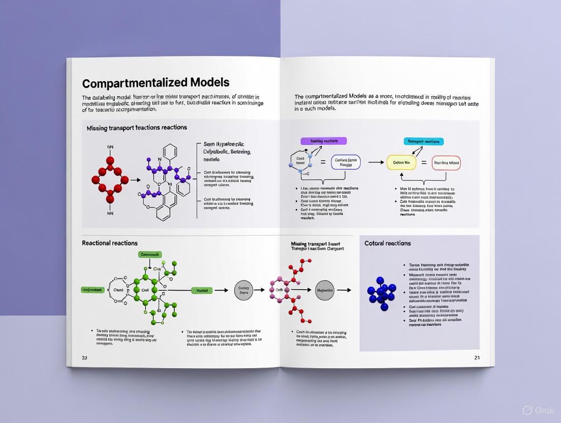
Overcoming the Transporter Gap: Strategies for Handling Missing Transport Reactions in Compartmentalized Metabolic Models
Accurate prediction of phenotype and cellular interactions using compartmentalized, constraint-based metabolic models is critically dependent on the completeness and accuracy of transporter annotations.
Overcoming the Transporter Gap: Strategies for Handling Missing Transport Reactions in Compartmentalized Metabolic Models
Abstract
Accurate prediction of phenotype and cellular interactions using compartmentalized, constraint-based metabolic models is critically dependent on the completeness and accuracy of transporter annotations. However, transporter functions are notoriously difficult to annotate, leading to pervasive gaps that undermine model predictive power. This article provides a comprehensive guide for researchers and drug development professionals on the foundational principles, methodological solutions, and validation frameworks for identifying and resolving missing transport reactions. We explore the root causes of annotation errors, detail state-of-the-art gap-filling and experimental-computational integration techniques, and present troubleshooting strategies for optimizing model performance. A comparative analysis of validation approaches equips practitioners to build more robust, predictive models, thereby enhancing applications in metabolic engineering, personalized medicine, and microbial ecology.
The Critical Challenge of Incomplete Transporter Annotations in Metabolic Models
Transporters are membrane proteins that move substances across cellular compartments, acting as gatekeepers that control a cell's interaction with its environment and other cells. In metabolic modeling, accurate annotation of these transporters is crucial, as they directly determine which nutrients a microbe can access, what byproducts it secretes, and how it interacts with neighboring cells. Inaccurate transporter annotations create a fundamental bottleneck that compromises the predictive power of genome-scale metabolic models (GEMs), leading to significant errors in predicting phenotypes ranging from microbial growth to drug targets. This technical support center provides troubleshooting guidance for researchers addressing these critical bottlenecks in their computational and experimental workflows [1].
Troubleshooting Guide: Common Transporter Annotation Errors
Table 1: Primary Error Types in Transporter Annotation and Their Impacts
| Error Type | Description | Prevalence in Draft Models* | Consequence for Model Prediction |
|---|---|---|---|
| Missing Assignments | A functional transporter is not annotated or included in the model. | 8.9% | Falsely limits the organism's metabolic capabilities; predicts no growth when growth should occur. |
| False Assignments | A transporter is assigned an incorrect substrate. | 16.2% | Allows implausible metabolic exchanges; predicts growth on incorrect nutrients. |
| Directionality Errors | The translocation direction (in/out) is incorrectly specified. | 4.5% | Reverses flux expectations; e.g., predicts secretion of a compound that should be imported. |
| GPR Mapping Errors | Incorrect gene-protein-reaction relationships (e.g., complex subunits). | Variable | Disconnects genotype from phenotype; hampers strain design and gene knockout predictions. |
*Data based on analysis of E. coli K12 MG1655, comparing a curated model (iML1515) vs. an automatically generated model (CarveMe). Error rates are likely higher for non-model organisms [1].
Diagnosis and Solutions for Annotation Errors
Problem: Model fails to predict growth on known carbon sources.
- Potential Cause: Missing transporter assignments for essential nutrients.
- Solution:
- Functional Cross-Checking: Use multiple annotation tools (see Table 2) and compare results. Do not rely on a single tool's output.
- Gap-filling Audit: Examine which transport reactions were gap-filled during model reconstruction. Manually curate these against experimental literature for the target organism or close phylogenetic relatives.
- Experimental Validation: Employ nutrient screening assays (e.g., Phenotype Microarrays) to experimentally confirm substrate uptake, then reconcile these results with the model.
Problem: Model predicts growth on substrates the organism cannot utilize.
- Potential Cause: False assignment of transporter substrate specificity.
- Solution:
- Substrate Specificity Check: Consult curated databases like TCDB for evidence of broad vs. narrow substrate specificity for the transporter family.
- Phylogenetic Analysis: Investigate if the substrate assignment is based on distant homologs with different functions. The substrate range can differ even within the same transporter family.
- Knockout Validation: If possible, compare predictions for a transporter gene knockout with experimental data for the same mutant.
Problem: Model accumulates internal metabolites or fails to secrete known byproducts.
- Potential Cause: Incorrect directionality or reversibility of transport reactions.
- Solution:
- Energetics Review: Check the thermodynamic constraints of the transport reaction (e.g., proton symport/antiport, ATP-coupled). This often dictates directionality.
- Literature Curation: Manually search for experimental evidence confirming the direction of transport in the specific organism.
- Compartment Localization: Verify that the enzyme producing the secreted metabolite is correctly localized to the same compartment as the transporter.
Frequently Asked Questions (FAQs)
Q1: Why are transporter annotations particularly problematic compared to other metabolic enzymes? Transporters present unique challenges due to several factors [1]:
- Non-Specific Substrate Assignments: Many are annotated with general terms (e.g., "ABC sugar transporter") without specific substrate information.
- Ambiguous Localization and Directionality: It is often unclear which membrane a transporter is located in and the direction in which it moves substrates.
- Complex Gene-Protein-Reaction Rules: They often form multi-subunit complexes (many-to-many mappings), making genetic basis difficult to define.
- Underground Metabolism: Promiscuous activity of transporters for non-canonical substrates is common but poorly annotated.
Q2: What are the best databases and tools for improving transporter annotations in my model? Table 2: Key Resources for Transporter Annotation and Functional Prediction
| Resource Name | Type | Key Features | URL |
|---|---|---|---|
| TCDB (Transporter Classification Database) | Curated Database | Gold-standard; uses TC system ontology; manually curated summaries. | www.tcdb.org |
| TransportDB | Computational Database | Phylogenetically broad; computationally derived; user-friendly portal. | www.membranetransport.org |
| TransAAP | Annotation Tool | Companion tool for TransportDB; performs automated annotation. | Integrated with TransportDB |
| ABCdb | Specialized Database | Focus on prokaryotic ATP-binding cassette (ABC) transporters. | www-abcdb.biotoul.fr |
| ARAMEMNON | Specialized Database | Focus on plant membrane proteins. | aramemnon.botanik.uni-koeln.de |
Q3: How can I account for spatial effects and compartmentalization in my transport models? Standard constraint-based models often assume a well-mixed cytoplasm. For more realistic spatial modeling, consider using specialized software like SMART (Spatial Modeling Algorithms for Reactions and Transport) [2]. SMART uses finite element analysis to solve mixed-dimensional partial differential equations, allowing you to model reaction-diffusion-transport processes in realistic 3D cellular geometries derived from microscopy data. This is critical for simulating gradients and localized signaling events that simple ODE-based models cannot capture.
Q4: My model is for a microbial community. How do transporters affect the prediction of cross-feeding interactions? Community interactions are almost entirely governed by transport. Metabolite exchange (cross-feeding), competition, and antagonism are all mediated by transporters. Inaccurate annotations will lead to:
- False Positive Interactions: Predicting a syntrophic relationship where one species provides a metabolite that the other cannot actually import.
- False Negative Interactions: Missing a key cross-feeding interaction because the importer is not annotated.
- Incorrect Dynamics: Misrepresenting the ecological outcome of the interaction. Rigorous curation of transport reactions is therefore the foundation of reliable community modeling [1].
Experimental Protocols for Validation
Protocol: High-Throughput Functional Characterization of Transporters
Objective: To experimentally determine the substrate specificity and uptake kinetics of orphan transporters.
Workflow:
Materials:
- Strain: Deletion mutant of a model organism (e.g., E. coli) lacking native transporters for the target substrate family.
- Vector: Expression plasmid with inducible promoter for cloning candidate transporter genes.
- Media: Defined minimal media with a single carbon/nitrogen/sulfur source candidate.
- Equipment: Plate reader for high-throughput growth curves, LC-MS/NMR for extracellular metabolomics.
Method:
- Clone the candidate transporter gene(s) into an expression vector.
- Transform the vector into a model host strain lacking the ability to transport a range of substrates.
- Culture the transformed strain in 96-well plates containing minimal media supplemented with a single candidate substrate. Include empty vector controls.
- Measure growth kinetics (OD600) over 24-48 hours. Significantly improved growth over the control indicates functional transport of the substrate.
- Confirm uptake by measuring the depletion of the substrate from the media using analytical techniques like LC-MS.
- Integrate confirmed substrates into the metabolic model with appropriate kinetic parameters if available.
Protocol: Computational Reconstruction of Transport Systems
Objective: To systematically add transport reactions to a draft genome-scale metabolic model.
Workflow:
Method:
- Automated Annotation: Run the target genome through annotation pipelines (e.g., TransAAP, RAST, ModelSEED) to generate a preliminary list of transporters and their putative substrates.
- Database Curation: Cross-reference this list with manually curated databases, primarily TCDB. Examine the family classification and any experimental evidence for substrates.
- Literature Mining: Perform a targeted search for biochemical characterization of the specific transporter or its close homologs.
- GPR Assignment: Define the gene-protein-reaction relationships, carefully accounting for protein complexes (e.g., ATP-binding and transmembrane subunits of ABC transporters).
- Compartmentalization: Assign the transporter to the correct membrane (e.g., cytoplasmic vs. periplasmic membrane in Gram-negative bacteria).
- Gap-filling: Use computational gap-filling tools as a starting point, but manually curate any added transport reactions for biological plausibility.
Table 3: Key Reagent Solutions for Transporter Research
| Reagent / Resource | Function / Application | Example / Specification |
|---|---|---|
| Heterologous Expression Hosts | Provides a clean background for characterizing orphan transporters. | E. coli BW25113 (ΔptsG, manZ, etc.) or S. cerevisiae BY4741 (Δhxt1-17). |
| Specialized Competent Cells | For efficient transformation of large or complex transporter gene constructs. | NEB 10-beta Competent E. coli (C3019) for large constructs; electrocompetent cells for high efficiency [3]. |
| Membrane Protein Purification Kits | Isolating functional transporters for in vitro assays. | Detergent-based kits with lipids to maintain protein stability (e.g., SMALPs). |
| Isotope-Labeled Substrates | Tracing uptake and flux through specific transporters. | 13C- or 14C-labeled glucose, amino acids; used in uptake assays and flux balance analysis. |
| Phenotype Microarray Plates | High-throughput profiling of metabolic capabilities, including transport. | Biolog PM plates (e.g., Carbon Source PM1 & PM2). |
| Finite Element Analysis Software | Spatial modeling of transport and reaction-diffusion processes. | SMART software package, built on FEniCS, for realistic cellular geometries [2]. |
Frequently Asked Questions
Q1: What is the most critical consequence of a missing transport reaction in a metabolic model?
- A1: A missing transport reaction can create a false prediction of thermodynamic infeasibility for an entire pathway that is known to function in vivo. The model may incorrectly block a flux-carrying pathway because an intermediate metabolite is effectively "trapped" in the wrong compartment, making the pathway appear non-functional [4].
Q2: How can a "false assignment" of an enzyme's location lead to errors in model predictions?
- A2: False localization assignments disrupt the model's spatial representation of metabolism. If an enzyme is annotated in a compartment where it does not exist, the associated reactions will not occur, potentially blocking pathways. Conversely, if it is missing from a compartment where it is active, the model may fail to account for metabolic flows that exist in the real cell, leading to inaccurate predictions of metabolite production or consumption [5].
Q3: What are the common sources of directionality issues in transport reactions?
- A3: Directionality issues often stem from incorrect thermodynamic constraints. If the Gibbs free energy (ΔG) of a transport reaction is not properly defined, the model may allow a reaction to proceed in a thermodynamically infeasible direction (e.g., pumping a metabolite against its concentration gradient without energy input). This can lead to the false prediction of energy-generating cycles or the infeasible accumulation of metabolites [4].
Q4: What is a "distributed bottleneck reaction," and how is it related to compartmentalization?
- A4: A distributed bottleneck is a set of reactions that, when considered together across compartments, become thermodynamically infeasible and limit pathway flux. This often occurs when a limiting metabolite is shared between these reactions. Properly modeling enzyme complexes and multifunctional enzymes as "compartments" can prevent these unrealistic distributed bottlenecks by ensuring that intermediate metabolites are channeled correctly [4].
Q5: Beyond metabolite trapping, what other model functionalities are affected by missing transport reactions?
- A5: Missing transport reactions can corrupt essential model analyses, including:
- Growth Prediction: Inaccurate biomass production due to missing essential nutrients or building blocks.
- Gene Essentiality Analysis: Incorrectly predicting a gene is non-essential because its reaction is compartmentalized and disconnected from the main network.
- Pathway Yield Calculation: Underestimating the maximum theoretical yield of a product by omitting key transport steps [4].
- A5: Missing transport reactions can corrupt essential model analyses, including:
Experimental Protocol: Validating Transport Reaction Annotations
This protocol provides a methodology for experimentally verifying the presence and directionality of a suspected transport reaction in a bacterial system, using serine synthesis as an example context [4].
1. Goal: To confirm the active transport of a metabolite (e.g., serine) across the cell membrane and characterize its kinetics.
2. Materials:
- Strain: Wild-type and mutant strain lacking the putative transporter gene.
- Culture Media: Defined minimal media with and without the target metabolite.
- Equipment: Spectrophotometer, HPLC system, rapid filtration apparatus, radiolabeled metabolite (e.g., ¹⁴C-Serine).
- Buffers: Appropriate washing and resuspension buffers.
3. Method:
Step 1: Growth Phenotype Assay
- Inoculate wild-type and transporter knockout strains into minimal media with the target metabolite as the sole carbon/nitrogen source.
- Monitor growth (OD₆₀₀) over time.
- Expected Outcome: Impaired growth of the knockout strain suggests a reliance on the transporter for metabolite uptake.
Step 2: Direct Transport Measurement
- Grow cells to mid-log phase and harvest.
- Wash and resuspend cells in a buffer with an energy source.
- Initiate transport by adding a radiolabeled metabolite (e.g., ¹⁴C-Serine).
- At timed intervals, aliquot cells and rapidly filter to separate cells from the medium.
- Wash filters and measure retained radioactivity via scintillation counting.
Step 3: Kinetic Analysis
- Repeat Step 2 with varying concentrations of the radiolabeled metabolite.
- Plot uptake rate versus substrate concentration to determine kinetic parameters (Km, Vmax).
Step 4: Efflux Assay
- Pre-load cells with the radiolabeled metabolite.
- Transfer cells to a metabolite-free buffer and monitor the disappearance of intracellular label and its appearance in the external medium over time.
4. Data Interpretation:
- Significantly higher uptake in the wild-type versus knockout confirms the transporter's function.
- Kinetic parameters define the efficiency and capacity of transport.
- Data from the efflux assay helps establish the reversibility or directionality of the transport reaction.
The Scientist's Toolkit: Research Reagent Solutions
Table: Key Reagents for Investigating Transport Reactions
| Reagent / Material | Function in Experiment |
|---|---|
| Radiolabeled Metabolites (e.g., ¹⁴C-Serine) | To trace and quantitatively measure the uptake and efflux of specific metabolites across the cell membrane with high sensitivity. |
| Gene Knockout Mutant Strains | To provide a comparative model where a specific transporter gene is deactivated, confirming the protein's role in the observed phenotype. |
| Defined Minimal Media | To create a controlled nutritional environment where the target metabolite can be presented as an essential growth factor, revealing transport dependencies. |
| Rapid Filtration Apparatus | To quickly separate bacterial cells from the external medium at precise time points, enabling accurate kinetic measurements of transport. |
| Constraints-Based Metabolic Model (e.g., EcoETM) | A computational model integrating enzymatic and thermodynamic constraints used to simulate metabolism and identify potential annotation errors by comparing predictions with experimental data [4]. |
Quantitative Data on Model Annotation Challenges
Table: Impact of Correcting Enzyme Compartmentalization on Pathway Predictions
The following data, derived from studies on the EcoETM model, summarizes how resolving enzyme compartmentalization and localization errors directly impacts model predictions for amino acid synthesis pathways [4].
| Pathway | Error Type | Model Prediction Before Correction | Model Prediction After Correction | Key Corrected Parameter |
|---|---|---|---|---|
| L-Serine Synthesis | Distributed Bottleneck (Unrealistic free intermediates) | Thermodynamically Infeasible (MDF < 0 kJ/mol) | Thermodynamically Feasible (MDF > 4 kJ/mol) | Treatment of PGCD, PGK, GAPD, FBA, TPI as a combined unit |
| L-Tryptophan Synthesis | Mis-localized or Non-compartmentalized Enzymes | Sub-optimal Yield & Flux | Maximum Theoretical Yield Achieved | Proper assignment of enzyme complexes (e.g., Aro complex) |
| General EMP Pathway | Distributed Bottleneck Reactions | False prediction of pathway incompatibility with L-Serine synthesis | Co-existence and integration of pathways is feasible | Consideration of multifunctional enzymes as reaction compartments |
Workflow Visualization for Error Deconstruction
Pathway Analysis with Corrected Compartmentalization
In the context of handling missing transport reactions in compartmentalized models, researchers frequently encounter the challenge of many-to-many (M:N) relationships between biological entities. These complex mappings—where multiple genes can correspond to multiple proteins, and multiple proteins can interact with multiple substrates—create significant hurdles in developing accurate metabolic and signaling models [1]. In compartmentalized biochemical pathways, understanding these relationships is crucial for predicting cellular behavior, as promiscuous protein interaction circuits perform critical computational functions within cells, especially in multicellular organisms [6]. This technical support guide addresses the specific issues researchers face when working with these complex systems and provides practical troubleshooting methodologies for your experiments.
FAQs: Addressing Common Experimental Challenges
How do I identify missing transport reactions in my metabolic model?
Missing transport reactions represent one of the most significant hurdles in constraint-based metabolic modeling, particularly for non-model organisms. These errors typically fall into three categories [1]:
- Missing assignments: The transporter is completely absent from your model
- False assignments: The model includes incorrect substrate-transporter relationships
- Directionality errors: Transport reactions are configured with incorrect import/export directions
In automatically generated genome-scale metabolic models (GEMs), approximately 30% of annotated transporter functions may contain errors. For well-studied organisms like E. coli K12 MG1655, error rates in draft models can include 8.9% missing assignments, 16.2% false assignments, and 4.5% directionality errors [1].
Troubleshooting protocol:
- Validate against curated models: Compare your model with extensively curated templates like iML1515 for E. coli
- Perform phylogenetic analysis: Check transporter annotations in closely related species
- Use multiple databases: Cross-reference with TCDB and TransportDB to identify potential missing transporters
- Test growth predictions: Compare in silico growth capabilities with experimental data under different nutrient conditions
What experimental approaches can resolve ambiguous E3 ligase-substrate relationships?
The ubiquitin-proteasome system exemplifies many-to-many relationships, with >600 E3 ubiquitin ligases potentially targeting numerous protein substrates. Traditional approaches like co-immunoprecipitation often fail to detect transient interactions [7].
Multiplex CRISPR screening workflow [7]:
- Create substrate library: Clone pools of peptide substrates or full-length ORFs as C-terminal fusions to GFP using the Global Protein Stability (GPS) platform
- Integrate CRISPR components: Clone a library of sgRNAs targeting E3 ligases into the same vector
- Transduce and select: Transduce Cas9-expressing cells at low MOI and select with puromycin
- Sort and sequence: Isolate stabilized cells via FACS, then perform paired-end sequencing to identify both substrate and sgRNA
This approach successfully performed ~100 CRISPR screens in a single experiment, correctly assigning C-terminal degrons to cognate adaptors like KLHDC2 (-GG* motifs) and APPBP2 (RxxG motifs) [7].
How can I accurately model compartmentalized systems with many-to-many relationships?
Compartmentalization fundamentally affects biochemical pathway dynamics, but standard ODE models may not adequately capture these effects. The spatial organization of pathways—with components distributed between membranes, cytoplasm, and organelles—is ubiquitous in both signaling and metabolic processes [5].
Model validation framework [5]:
- Develop PDE description: Create reaction-diffusion equations accounting for compartment boundaries
- Define compartment-specific kinetics: Implement distinct reaction terms for each compartment
- Establish conservation rules: Specify total amounts of conserved species when solving for steady states
- Compare with ODE models: Validate whether simplified compartmental ODE models can reasonably capture system behavior
For a two-compartment system with diffusive transport, the PDE description would include:
- In compartment 1 (θ ∈ Ω₁): ∂Xⱼ/∂t = fⱼ₁(X₁, X₂, ..., Xₙ) + Dⱼ(∂²Xⱼ/∂θ²)
- Between compartments (θ ∈ Ω₁₂): ∂Xⱼ/∂t = Dⱼ(∂²Xⱼ/∂θ²)
- In compartment 2 (θ ∈ Ω₂): ∂Xⱼ/∂t = fⱼ₂(X₁, X₂, ..., Xₙ) + Dⱼ(∂²Xⱼ/∂θ²)
Key Data Tables for Experimental Planning
Table 1: Transporter Annotation Error Rates in Metabolic Models
| Error Type | Description | Frequency in E. coli Draft Models | Impact on Model Predictions |
|---|---|---|---|
| Missing Assignments | Transporter completely absent from model | 8.9% | Exclusion of metabolic reactions, incorrect gap-filling |
| False Assignments | Incorrect substrate-transporter relationships | 16.2% | Prediction of impossible metabolic capabilities |
| Directionality Errors | Incorrect import/export direction | 4.5% | Violation of thermodynamic constraints |
| Total Error Rate | ~30% | Significant impact on phenotype prediction accuracy |
Table 2: Genetic Interaction Enrichment in Protein Complexes
| Interaction Type | Interaction Score Threshold | Enrichment in Known Complexes | Biological Significance |
|---|---|---|---|
| Physical Interactions | PE-score > 5 | ~50-fold enrichment | Direct physical association in complexes |
| Alleviating Genetic Interactions | S-score > +2.5 | ~100-fold enrichment | Functional compensation within complexes |
| Aggravating Genetic Interactions | S-score < -2.5 | ~100-fold enrichment | Essential gene enrichment in complexes |
| Random Protein Pairs | - | 1-fold (baseline) | Negative control for comparison |
Experimental Protocols
Comprehensive Transporter Annotation Protocol
Purpose: To accurately identify and characterize transport reactions for metabolic models of non-model organisms.
Materials:
- Genomic data for target organism
- Curated metabolic models for phylogenetically related organisms
- Transporter classification databases (TCDB, TransportDB)
- Functional annotation tools (TransAAP, CarveMe)
Methodology [1]:
- Initial annotation: Use multiple automated tools to generate transporter annotations
- Database cross-referencing: Compare results against TCDB (manually curated) and TransportDB (computationally derived)
- Phylogenetic profiling: Identify conserved transporters in related species
- Manual curation: Resolve conflicts between automated annotations based on literature evidence
- Gap analysis: Identify potentially missing transporters based on metabolic capabilities
- Experimental validation: Design growth assays to test transporter predictions
Troubleshooting tips:
- For organisms distant from well-studied models, expect higher error rates in automated annotations
- Pay particular attention to transporter directionality and energy coupling mechanisms
- Account for "moonlighting" proteins with multiple functions and promiscuous activities
Integrated Genetic-Physical Interaction Mapping
Purpose: To identify functional modules and relationships by combining genetic interaction and physical binding data.
Materials:
- Quantitative genetic interaction data (E-MAP or SGA)
- Physical interaction data (TAP-MS or co-IP)
- Protein complex databases (MIPS, CORUM)
- Computational integration framework
Methodology [8]:
- Data integration: Combine quantitative genetic interaction scores (S-scores) with physical interaction confidence scores (PE-scores)
- Module detection: Identify sets of proteins that interact physically more than expected by chance
- Functional relationship mapping: Establish connections between modules based on genetic interaction patterns
- Validation: Compare identified modules against known complexes in benchmark datasets
Key analysis [8]:
- Protein pairs with extreme S-scores (both positive and negative) show ~100-fold enrichment in known complexes
- Strong physical interactions (high PE-scores) show ~50-fold enrichment
- This approach has demonstrated >50% improved accuracy in identifying functionally related protein pairs compared to previous methods
Essential Visualizations
Many-to-Many Relationships in Biological Systems
Multiplex CRISPR Screening Workflow
Compartmentalized Reaction-Diffusion System
The Scientist's Toolkit: Research Reagent Solutions
Table 3: Essential Research Materials for Mapping Complex Relationships
| Reagent/Resource | Primary Function | Application Context | Key Features |
|---|---|---|---|
| GPS Platform | Simultaneous stability profiling of substrate pools | E3 ligase-substrate identification | GFP-fusion libraries with DsRed internal control |
| TCDB Database | Transporter classification and annotation | Metabolic model refinement | Manually curated, IUBMB-recognized ontology |
| Multiplex CRISPR Vector | Combined substrate expression and gene knockout | High-throughput E3-substrate mapping | Integrated GPS and sgRNA expression cassettes |
| E-MAP Technology | Quantitative genetic interaction measurement | Functional relationship mapping | Continuous growth rates with epistasis scoring |
| TransportDB | Computational transporter annotation | Initial metabolic model generation | Covers 2,761 organisms with web interface |
| CARVEME | Automated metabolic model reconstruction | Draft model generation | Reference-based gap filling |
Frequently Asked Questions
1. What are the primary causes of incorrect transporter annotations in metabolic models? Incorrect annotations primarily stem from three types of errors [1]:
- Missing Assignments: A transporter exists in the organism but is not annotated in the model.
- False Assignments: A transporter is annotated with an incorrect substrate.
- Directionality Errors: The annotated direction of transport (e.g., import vs. export) does not match the biological function. These errors are compounded by the complex "many-to-many" relationships between transporter genes, the proteins they encode, and the multiple substrates they can carry [1].
2. How can I identify a transporter of unknown function in a newly sequenced genome?
The Transporter Classification Database (TCDB) offers specialized tools for this purpose. The findNovelTransporters program is designed to scan a genome and identify potential transmembrane proteins that show little or no sequence similarity to any known transporter in TCDB, helping to pinpoint novel transporter families [9].
3. My model is missing transport reactions for a key nutrient. What is a reliable workflow to address this? A reliable protocol involves a multi-step, iterative process of bioinformatic prediction and experimental validation, as outlined below [1]:
4. Why is TCDB considered the international standard for transporter classification? The Transporter Classification Database (TCDB) is the only database adopted by the International Union of Biochemistry and Molecular Biology (IUBMB) as the officially recognized system for classifying transport proteins [9] [1]. Its system is based on a hierarchy that considers the transporter's mechanism, energy coupling, and phylogenetic relationships, providing a consistent framework for researchers worldwide [9].
5. What is the key difference between the curation approaches of TCDB and TransportDB? TCDB is a manually curated database where each entry is supported by literature and detailed summaries [1]. In contrast, TransportDB provides computationally derived annotations for a large number of organisms (over 2,700) using its TransAAP tool, which automates the prediction of transporter families [1].
The Scientist's Toolkit: Research Reagent Solutions
| Resource Name | Type | Primary Function | Key Feature |
|---|---|---|---|
| TCDB (tcdb.org) [9] [1] | Curated Database | Classification & functional data for transporters. | IUBMB-recognized ontology; detailed manual curation. |
| TransportDB 2.0 [1] | Computational Database | Genome-scale prediction & annotation of transporters. | User-friendly portal; pre-computed for many genomes. |
| ModelSEED [10] | Modeling Platform | Automated construction & analysis of metabolic models. | Integrates annotation data to build genome-scale models. |
| GBlast [9] | Bioinformatics Tool | Comparative genomic analysis to identify transporter homologs. | Part of the TCDB software suite. |
| TransAAP [1] | Annotation Tool | Automated annotation of transporter families in genomic data. | Powers the predictions in TransportDB. |
| FEniCS [2] | Simulation Platform | Solves spatial reaction-transport equations in complex geometries. | Used for compartmentalized modeling in tools like SMART. |
Quantitative Database Comparison
The following table summarizes the core quantitative and qualitative attributes of the key databases as of late 2020/2024.
| Feature | TCDB [9] [1] | TransportDB [1] | ModelSEED [10] |
|---|---|---|---|
| Primary Focus | Classification & Curation | Genomic Prediction | Metabolic Model Reconstruction |
| Curation Style | Manual | Computational | Computational & Manual Curation |
| Classification System | TC System (IUBMB) | Based on TC System & Other Ontologies | Biochemical Reaction Network |
| Number of Organisms | Not Specified (Family-centric) | 2,761 (Predominantly Bacteria) | Integrated into Models |
| Number of Proteins/Systems | 20,653 proteins in 15,528 systems [9] | Not Specified | N/A |
| Number of Families | 1,536 [9] | Not Specified | N/A |
| 3D Structures | 1,567 with PDB accessions [9] | Not Specified | N/A |
| Key Tools | GBlast, famXpander, singEasy [9] | TransAAP [1] | ModelSEEDpy, ProbAnno [10] |
Experimental Protocol: Validating Transporter Function
Objective: To experimentally confirm the substrate and directionality of a putative sugar transporter gene (sugT) identified bioinformatically in a bacterial genome.
Background: Accurate annotation is critical. A study on E. coli found that automatically generated models can have error rates over 30% for transporter functions, including false and missing assignments [1]. This protocol outlines a validation workflow.
Materials:
- Wild-type bacterial strain and ΔsugT knockout strain (created via gene deletion).
- M9 minimal growth media with various candidate sugars (e.g., glucose, xylose, fructose) as sole carbon sources.
- Shaking incubator and spectrophotometer for growth curve analysis.
- LC-MS/MS instrumentation for quantifying extracellular and intracellular metabolite levels.
Methodology:
- Knockout Strain Generation: Create a clean deletion of the
sugTgene in the wild-type background using standard genetic techniques (e.g., allelic exchange). - Growth Phenotype Screening: Inoculate wild-type and ΔsugT strains into M9 media supplemented with individual candidate sugars. Monitor optical density (OD) over 24-48 hours to generate growth curves.
- Metabolite Uptake/Secretion Assay:
- Grow both strains to mid-exponential phase in a rich medium.
- Harvest, wash, and resuspend cells in a buffer containing the target sugar.
- Take samples from the supernatant at regular intervals.
- Use LC-MS/MS to quantify the concentration of the sugar in the supernatant over time. A slower decrease in concentration for the knockout indicates impaired import.
- Data Integration into Model:
- Map the confirmed substrate and import directionality to the
sugTgene in the metabolic reconstruction. - Ensure the model can simulate growth on the validated sugar and fails to do so when the corresponding transport reaction is removed.
- Map the confirmed substrate and import directionality to the
The logical flow of this experimental design is summarized in the following diagram:
Practical Solutions: From Automated Gap-Filling to Integrated Experimental-Computational Workflows
Frequently Asked Questions
What is metabolic gap-filling and why is it necessary? Genome-scale metabolic models (GSMMs) are often incomplete due to genome misannotations and unknown enzyme functions, leading to metabolic gaps—dead-end metabolites or pathways that prevent the model from simulating known metabolic functions, such as growth on a specific carbon source [11] [12]. Gap-filling is a computational process that adds biochemical reactions from external databases to the metabolic reconstruction to restore network connectivity and model functionality [11].
My model is not growing after gap-filling. What could be wrong? This is often the core problem gap-filling aims to solve. If growth is not restored, consider these points:
- Insufficient Reactions: The universal reaction database used may lack the necessary reactions to complete the essential metabolic pathway [13].
- Incorrect Objective: Ensure the model's objective (e.g., biomass production) is correctly set as the target for the gap-filling algorithm [13].
- Community Context: For organisms that live in microbial communities, a community-level gap-filling approach that allows metabolic interactions between species may be required to resolve gaps that cannot be filled using a single-species model [11].
The gap-filling MILP solver is taking too long and not converging. How can I optimize it? Mixed-integer Linear Programming (MILP) for gap-filling is computationally expensive [13]. Performance issues can be mitigated by:
- Reformulating the Problem: Using more efficient algorithms like
FASTGAPFILLorGLOBALFIT, which reformulate the MILP into a simpler Linear Programming (LP) or bi-level optimization problem to decrease solution times [11] [12]. - Solver Choice: Open-source solvers may struggle with larger models; commercial solvers like Gurobi or CPLEX can offer significant speed improvements [14].
- Model Tightening: Improve the formulation by tightening the bounds of continuous variables, breaking symmetry in the model, and ensuring all variables have bounds [14].
- Reformulating the Problem: Using more efficient algorithms like
What is the difference between single-species and community-level gap-filling? Traditional gap-filling algorithms resolve gaps in a single organism's model in isolation [12]. Community-level gap-filling integrates incomplete metabolic reconstructions of multiple microorganisms known to coexist. It allows them to interact metabolically (e.g., through cross-feeding) during the gap-filling process, which can resolve gaps in a more biologically realistic way for interdependent species and predict non-intuitive metabolic interdependencies [11].
How do I validate gap-filling predictions experimentally? Gap-filling predictions generate hypotheses that require experimental validation [12]. Key approaches include:
- High-Throughput Phenotyping: Testing model predictions of growth phenotypes under different nutrient conditions or for knockout mutants [12].
- Biochemical Assays: Directly testing the enzymatic activity of a gene product predicted to fill a metabolic gap [12].
- Genetic Complementation: Expressing a predicted gene in a mutant strain that lacks the corresponding function to see if it restores growth [12].
Experimental Protocols for Gap-Filling Validation
Protocol for Community-Level Gap-Filling and Cross-Feeding Validation
This methodology is adapted from studies on synthetic E. coli communities and human gut microbiota consortia [11].
- Objective: To resolve metabolic gaps in a model by leveraging metabolic interactions between two or more microbial species and validate predicted cross-feeding.
Materials:
- Incomplete GSMMs for the target organisms (e.g., Bifidobacterium adolescentis and Faecalibacterium prausnitzii).
- A reference biochemical reaction database (e.g., MetaCyc, ModelSEED).
- Constraint-based modeling software with gap-filling capabilities (e.g., Cobrapy [13]).
- Anaerobic growth chamber, defined growth media, and analytical equipment (e.g., HPLC for measuring metabolite concentrations).
Procedure:
- Model Compartmentalization: Create a community metabolic model by combining the individual GSMMs of each species into a single model, adding an extracellular compartment for metabolite exchange [11].
- Define Community Objective: Set a community-level objective function, such as the total biomass of all species.
- Run Community Gap-Filling: Apply a community gap-filling algorithm that permits the addition of reactions from the database to any species' model within the community to achieve the community objective [11]. The algorithm minimizes the total number of added reactions.
- In Silico Prediction: Simulate the gap-filled community model to predict growth rates and metabolic cross-feeding (e.g., acetate secretion by one species and its consumption by another).
- In Vitro Validation:
- Cultivate each species individually in defined media to confirm their auxotrophies.
- Co-culture the species in the same media and monitor community growth and metabolite concentrations over time.
- Compare the measured metabolite cross-feeding (e.g., using HPLC) and growth yields with the model's predictions [11].
Protocol for Resolving False-Negative Growth Predictions in a Single Species
This protocol addresses the common gap-filling scenario where a model fails to simulate growth on a known carbon source [12].
- Objective: To identify and fill missing reactions that enable an organism to grow on a specific substrate.
Materials:
- The incomplete GSMM.
- A universal model of biochemical reactions.
- Experimental data on the organism's ability to grow on the target substrate.
Procedure:
- Detect the Gap: Set the model's objective to growth and the environment to allow only the target substrate as a carbon source. A growth rate of zero indicates a gap [13].
- Formulate the MILP Problem: The gap-filling algorithm is formulated to find the minimal set of reactions from the universal model that, when added, enables growth. The objective is to minimize the sum of the costs of the added reactions [13]: Minimize: ( \sumi ci * zi ) Subject to: ( Sv = 0 ) (Mass balance constraints) ( v^\star \geq t ) (Growth constraint, where ( v^\star ) is the flux of the biomass reaction and ( t ) is a lower bound) ( li \leq vi \leq ui ) (Flux bounds for each reaction ( i )) ( vi = 0 \textrm{ if } zi = 0 ) (Reaction ( i ) is inactive if not selected)
- Execute Gap-Filling: Solve the MILP to obtain one or multiple possible reaction sets that restore growth [13].
- Gene Assignment: Use bioinformatics tools (e.g., sequence similarity, phylogenetic profiling) to propose candidate genes in the organism's genome that could catalyze the gap-filled reactions [12].
- Experimental Testing: Genetically knock out the predicted gene and assay for loss of growth on the target substrate, or heterologously express the gene to prove its function [12].
Gap-Filling Algorithm Standards and Performance Metrics
The following table summarizes key quantitative standards and metrics for evaluating gap-filling algorithms, as established in the field [11] [12].
Table 1: Key Performance Metrics for Gap-Filling Algorithms
| Metric | Description | Typical Target or Value |
|---|---|---|
| Computational Efficiency | Time to find a solution; scalability to genome-scale models. | LP formulations (e.g., FASTGAPFILL) are faster than MILP [11] [12]. |
| Solution Accuracy | Ability to recover known metabolic functions and pathways. | Validated by predicting experimentally confirmed growth phenotypes [12]. |
| Solution Minimality | Number of reactions added to the model to restore functionality. | Algorithms aim for the smallest possible set of added reactions [11] [13]. |
| Gene Assignment Accuracy | For algorithms that suggest genes, the correctness of the gene-protein-reaction (GPR) association. | Assessed via genetic or biochemical experiments (e.g., knockout mutants) [12]. |
Research Reagent Solutions
This table lists essential computational and biological reagents used in gap-filling research.
Table 2: Essential Reagents for Gap-Filling Research
| Reagent / Tool | Function in Gap-Filling Research |
|---|---|
| Genome-Scale Metabolic Model (GSMM) | A mathematical representation of an organism's metabolism; the substrate for gap-filling analysis [11] [15]. |
| Universal Biochemical Database (e.g., MetaCyc, ModelSEED) | A reference set of known biochemical reactions used as a source for candidate reactions to fill metabolic gaps [11] [13]. |
| Constraint-Based Modeling Software (e.g., Cobrapy) | Provides the computational environment to simulate metabolism, detect gaps, and implement gap-filling algorithms [13]. |
| Defined Growth Media | Used in vitro to validate model predictions by testing growth of wild-type and mutant strains under specific nutrient conditions [11] [12]. |
Workflow and Relationship Visualizations
Gap-Filling Core Workflow
The following diagram illustrates the standard iterative process for developing and validating a genome-scale metabolic model through gap-filling [11] [12].
Community vs Single-Species Gap-Filling
This diagram contrasts the traditional single-species gap-filling approach with the community-level approach, highlighting the key difference of allowing metabolic interactions [11].
Frequently Asked Questions (FAQs)
What is the primary goal of gap-filling a metabolic model?
The goal of gap-filling is to identify a minimal set of biochemical reactions that, when added to a draft genome-scale metabolic model (GEM), enable it to produce all essential biomass precursors from a specified set of nutrient compounds in the growth media. This process compensates for knowledge gaps arising from incomplete genomic annotations or uncharacterized enzyme functions, thereby restoring network connectivity and enabling computationally simulated growth [16] [11] [17].
Why is the choice of growth media condition critical for the gap-filling process?
The media condition defines the metabolites available for uptake by the model. Consequently, it directly determines which metabolic pathways must be complete and functional for the organism to synthesize all biomass components. Gap-filling on a minimal media will force the algorithm to add reactions for the de novo biosynthesis of many essential metabolites. In contrast, gap-filling on a rich or complete media allows the algorithm to simply add transport reactions for metabolites that are already present in the environment, potentially resulting in a model with fewer biosynthetic capabilities that is dependent on a nutrient-rich setting. The choice of media should therefore reflect the known physiological conditions of the organism [16].
What is "Complete" media in KBase and when should I use it?
In platforms like KBase, "Complete" media is an abstraction that includes every compound in the biochemistry database for which a transport reaction exists. It is not a stored object but is built in real-time when selected. While useful as a starting point to see if a model can grow under ideal, nutrient-rich conditions, gap-filling on Complete media often results in the addition of numerous transport reactions and may not yield a physiologically realistic model. It is generally recommended for initial tests, but gap-filling on a defined, minimal media is better for constructing a robust, metabolically self-sufficient model [16].
How can I see which compounds are in a media condition?
Within KBase, you can view the compounds that comprise a media condition by opening the model viewer, selecting the 'Compounds' tab, and filtering the compartment to "e0" (which denotes the extracellular compartment). This will display a complete list of transportable compounds for your model under that specific media condition [16].
Troubleshooting Guides
Problem: Gap-filled Model is Not Growing on a New Media
Issue: A model that was successfully gap-filled on one media condition fails to simulate growth when switched to a different, well-defined media. Solution:
- Stack Gap-filling Runs: Use the original, non-gapfilled draft model for all new gap-filling exercises. If you gap-filled on Complete media first and then want to adapt the model to a minimal media, do not use the already gap-filled model. Instead, use the original draft model and perform a new, independent gap-filling run with the minimal media condition [16].
- Verify Media Composition: Double-check that the new media condition contains all essential nutrients, such as carbon, nitrogen, phosphorus, and sulfur sources, required by the target organism.
- Re-gapfill: Run the gap-filling app again on the original draft model, specifying the new target media. This will find a minimal set of reactions enabling growth on that specific media.
Problem: Gap-filling Solution Contains Biologically Irrelevant Reactions
Issue: The reactions proposed by the automated gap-filling algorithm are not biologically plausible for the organism being modeled (e.g., a reaction from a non-existent pathway or a thermodynamically infeasible direction). Solution:
- Manual Curation: Automated gap-filling is a heuristic, and its solutions require manual validation. After gap-filling, you can inspect the added reactions and use the "Custom flux bounds" field to force a biologically incorrect reaction to zero flux. Re-running the gap-filling will then force the algorithm to find an alternative solution [16].
- Leverage Physiological Data: Use known physiological data (e.g., preferred carbon sources, known secretion products) to guide the selection of media and to critically evaluate the gap-filling results. Studies have shown that manual curation incorporating expert biological knowledge significantly improves model accuracy [17].
- Refine the Draft Model: Ensure the draft model is as complete as possible before gap-filling. Using RAST for genome annotation, which provides a controlled vocabulary for functional roles, is recommended over other annotators like Prokka for metabolic modeling in KBase, as it improves the quality of the initial reaction network [16].
Problem: Inconsistent Phenotype Predictions After Gap-Filling
Issue: The gap-filled model generates false positives (predicts growth where it doesn't occur) or false negatives (fails to predict growth where it does occur). Solution:
- Validate with Experimental Data: Compare model predictions against experimental growth phenotyping data, if available. Discrepancies can highlight areas where the model requires further curation.
- Community-Level Gap-Filling: For models of organisms that live in complex microbial communities, consider using a community gap-filling algorithm. This method resolves gaps simultaneously across multiple metabolic models by allowing them to interact and exchange metabolites, which can lead to more accurate predictions of metabolic interactions and growth capabilities [11].
- Explore Advanced Methods: If phenotypic data is scarce, topology-based gap-filling methods like CHESHIRE can be used. These machine learning approaches predict missing reactions purely from the structure of the metabolic network and have been shown to improve predictions of fermentation products and amino acid secretion [18].
Media Selection Decision Workflow
The following diagram illustrates the logical process for selecting an appropriate media condition for gap-filling.
Research Reagent Solutions
The table below lists key resources and databases essential for conducting gap-filling analyses.
| Item Name | Type | Function in Gap-Filling |
|---|---|---|
| KBase Gapfill App [16] | Software Tool | A platform implementation that automates the gap-filling process using linear programming to find a minimal set of reactions to enable model growth. |
| ModelSEED Biochemistry [16] [11] | Reaction Database | A comprehensive database of biochemical reactions and compounds used as a reference set from which reactions are proposed during the gap-filling process. |
| BiGG Models [18] [11] | Reaction Database | A knowledgebase of curated, genome-scale metabolic models and a standardized reaction database used for reconstruction and gap-filling. |
| MetaCyc [11] [17] | Reaction Database | A curated database of metabolic pathways and enzymes often used as a reference repository of known biochemical reactions for gap-filling. |
| CarveMe [18] [11] | Software Tool | A tool for automated reconstruction of genome-scale metabolic models, which incorporates its own gap-filling algorithm. |
| SCIP / GLPK [16] | Solver | The optimization solvers used internally by gap-filling algorithms to solve the linear programming (LP) or mixed-integer linear programming (MILP) problems. |
| CHESHIRE [18] | Software Tool | A deep learning-based method that predicts missing reactions using only metabolic network topology, useful when phenotypic data is unavailable. |
| Community Gap-Filling Algorithm [11] | Methodology | A computational approach that resolves metabolic gaps across multiple models simultaneously by allowing metabolic interactions between community members. |
Step-by-Step Guide to Semi-Automated Model Reconstruction and Compartmentalization
This guide addresses the critical challenge of handling missing transport reactions during the reconstruction of compartmentalized, genome-scale metabolic models (GEMs). GEMs are mathematical representations of an organism's metabolism that integrate genes, proteins, and biochemical reactions [19]. Compartmentalization is the process of defining distinct subcellular locations (e.g., cytosol, mitochondria) within the model, which requires the accurate inclusion of transport reactions to move metabolites between these compartments. Gaps, or missing knowledge, in these transport networks are a primary source of model incompleteness, preventing accurate simulation of metabolic phenotypes [18] [20].
This technical support document provides a step-by-step protocol and troubleshooting guide to help researchers identify and resolve these gaps, thereby refining their models for more reliable predictions in drug target identification and metabolic engineering.
The Semi-Automated Reconstruction Workflow
The following diagram illustrates the comprehensive, multi-stage pipeline for reconstructing a high-quality, compartmentalized metabolic model, from initial draft creation to functional validation.
Detailed Experimental Protocols
Stage 1: Creating a Draft Reconstruction
Objective: To build an initial, genome-wide draft of the metabolic network.
- Genome Annotation: Begin with an annotated genome sequence. Use automated annotation servers like RAST or the SEED database to identify protein-coding genes and infer metabolic functions [21] [19].
- Generate Gene-Protein-Reaction (GPR) Associations: Link genes to the reactions they catalyze. This can be done automatically via pipelines like ModelSEED or by performing homology searches (e.g., BLAST) against well-curated template models (e.g., E. coli, B. subtilis) [21] [19].
- Define Biomass Objective Function: Assemble a biomass equation representing the composition of a new cell. This includes percentages of macromolecules like proteins, DNA, RNA, lipids, and other cellular components. This equation will serve as a key objective function for later simulations [21] [19].
Stage 2: Manual Curation and Compartmentalization
Objective: To refine the draft model by defining subcellular compartments and adding the requisite transport reactions.
- Assign Subcellular Localization: Predict the localization of enzymes using tools like PSORT or PA-SUB. This information is crucial for assigning reactions to the correct compartment (e.g., cytosol, mitochondria, periplasm) [19].
- Add Compartment-Specific Reactions: Review the reaction list and ensure all reactions are assigned to their correct subcellular location based on enzyme localization data.
- Add Intracellular Transport Reactions: For metabolites that are synthesized in one compartment and consumed in another, add specific transport reactions (e.g., antiport, symport, or ATP-driven transport) to enable inter-compartmental metabolite exchange. Consult transport-specific databases like the Transport Classification Database (TCDB) for this purpose [19].
Stage 3: Gap Analysis and Filling
Objective: To identify and resolve network gaps, with a special focus on missing transport reactions that disrupt connectivity between compartments.
- Identify Topological Gaps: Use computational tools like the
gapAnalysisfunction in the COBRA Toolbox to detect dead-end metabolites (metabolites that can only be produced or consumed, but not both) and blocked reactions (reactions that cannot carry any flux under any condition) [21] [20]. Dead-end metabolites are often a primary indicator of missing transport reactions. - Identify Phenotypic Inconsistencies: Compare model predictions with experimental data, such as known growth capabilities on different nutrient sources or gene essentiality data. Inconsistencies often point to network gaps [20].
- Fill Gaps: Add reactions from universal biochemical databases (e.g., KEGG, BRENDA) to resolve the identified gaps. The goal is to add a minimal set of reactions that allows the model to produce all essential biomass precursors and match known phenotypic data [21] [20]. Advanced, topology-based methods like CHESHIRE can also be employed to predict missing reactions purely from network structure [18].
Stage 4: Model Conversion and Simulation
Objective: To convert the curated reconstruction into a computable model and simulate metabolic behavior.
- Convert to Mathematical Model: Assemble the stoichiometric matrix (S), where rows represent metabolites and columns represent reactions. The matrix elements are the stoichiometric coefficients for each metabolite in each reaction [19].
- Set Constraints: Apply constraints to reaction fluxes (
v), defining their lower and upper bounds (v_j,minandv_j,max). These constraints represent known physiological limitations, such as nutrient uptake rates [21] [19]. - Perform Flux Balance Analysis (FBA): Use linear programming to solve the system
S • v = 0(assuming a steady state) and find a flux distribution that maximizes or minimizes a given objective function, most commonly the biomass reaction [21] [19].
Stage 5: Validation and Iterative Refinement
Objective: To ensure the model's predictions are biologically accurate.
- Compare Predictions: Systematically compare FBA predictions (e.g., growth rates, byproduct secretion, gene essentiality) against experimental data collected under defined conditions [21].
- Debug and Refine: If predictions disagree with experimental data, return to previous stages to curate GPR rules, adjust compartmentalization, or fill additional gaps. This is an iterative process until model performance is satisfactory [19].
FAQs & Troubleshooting Guides
Frequently Asked Questions
Q1: What are the most common types of gaps in a compartmentalized model? The most frequent gaps are dead-end metabolites and blocked reactions. In a compartmentalized model, a dead-end metabolite often appears when a metabolite is produced in one compartment but lacks a transport reaction to move it to the compartment where it is consumed. Blocked reactions are reactions that cannot carry flux because one or more of their reactants cannot be produced, or their products cannot be consumed, which can also be a consequence of missing transport [20].
Q2: My model fails to produce biomass in simulation. What is the first thing I should check?
First, perform a gap-filling analysis focused on biomass precursor synthesis. Use tools like gapFind to identify which biomass precursors cannot be synthesized. Check the pathways and transport reactions leading to the production of these specific precursors. Often, the issue is a missing transport reaction for a critical cofactor or building block [20].
Q3: How can I predict missing transport reactions when experimental data is scarce? You can use topology-based gap-filling methods that do not require experimental phenotypes. Methods like CHESHIRE use machine learning on the structure of the metabolic network itself to predict missing reactions, including transport reactions, with high confidence [18].
Q4: What is the difference between a draft model from an automated pipeline and a manually curated one? Automated pipelines (e.g., ModelSEED) provide a fast, first-pass reconstruction but often contain errors in GPR associations, reaction directionality, and lack compartmentalization and specific transport reactions. Manual curation, while time-consuming, is essential for resolving these issues, adding organism-specific details, and ensuring model accuracy and predictive power [21] [19].
Troubleshooting Common Issues
Problem: The model predicts growth where it shouldn't (False Positive).
- Potential Cause: The model may be missing regulatory constraints or contain an incomplete biomass definition that allows "energy-generating cycles" without actual growth.
- Solution:
- Verify the composition and stoichiometry of your biomass objective function.
- Check for and eliminate thermodynamically infeasible cycles.
- Integrate transcriptomic data to constrain reactions that should not be active under the simulated condition.
Problem: The model fails to predict growth where it should (False Negative).
- Potential Cause: This is a classic symptom of a gap in the network. A required reaction or, more specifically, a transport reaction for a key nutrient or metabolite is missing.
- Solution:
- Perform thorough gap analysis to find dead-end metabolites and blocked reactions.
- Ensure transport reactions for all essential nutrients in your growth medium are present and active.
- Use a gap-filling algorithm like SMILEY or GAUGE that utilizes experimental growth data to pinpoint and resolve the inconsistency [20].
Problem: A metabolite is "trapped" in one compartment.
- Potential Cause: A missing intracellular transport reaction.
- Solution:
- Identify the metabolite and its compartments of production and consumption.
- Query transport databases (TCDB) for known transporters for this metabolite.
- If a known transporter exists, add the corresponding reaction to your model. If not, you may need to add a generic exchange reaction as a placeholder for an unknown transport mechanism.
Computational Methods for Gap Filling
Several computational methods have been developed to aid the gap-filling process. The table below summarizes key approaches, the type of data they utilize, and their primary strategy.
Table 1: Comparison of Gap-Filling Methods for Metabolic Models
| Method Name | Type of Input Data | Optimization Algorithm | Primary Strategy |
|---|---|---|---|
| FastGapFill [20] | Topology (Blocked reactions) | Linear Programming (LP) / Mixed Integer Linear Programming (MILP) | Minimize number of added reactions from a database. |
| SMILEY [20] | Growth phenotype data | MILP | Minimize added reactions to allow growth on known carbon sources. |
| GrowMatch [20] | Gene essentiality data | MILP | Minimize added reactions to correct essentiality predictions. |
| CHESHIRE [18] | Network Topology Only | Deep Learning | Predict missing reactions via hypergraph learning, no experimental data needed. |
| GAUGE [20] | Gene Expression Data | MILP | Minimize discrepancy between flux coupling and gene co-expression by adding reactions. |
Decision Framework for Selecting a Gap-Filling Method
The logic for choosing an appropriate gap-filling strategy based on data availability and problem type is outlined below.
Table 2: Key Resources for Metabolic Model Reconstruction and Curation
| Category | Item / Tool | Function & Purpose |
|---|---|---|
| Genome Databases | RAST, NCBI Entrez, SEED | Automated genome annotation and functional assignment of genes [19]. |
| Biochemical Databases | KEGG, BRENDA, TCDB | Reference databases for biochemical reactions, enzyme properties, and transport reaction classification [19] [20]. |
| Template Models | BiGG Models, EcoCyc | High-quality, curated metabolic models used for homology-based reconstruction and GPR transfer [21] [19]. |
| Reconstruction Software | COBRA Toolbox, ModelSEED | Software suites providing functions for model reconstruction, simulation, gap-filling, and analysis [21] [19]. |
| Simulation Solver | GUROBI, CPLEX | Mathematical optimization solvers used to perform FBA and other constraint-based analyses [21]. |
| Localization Prediction | PSORT, PA-SUB | Tools to predict subcellular localization of proteins, critical for compartmentalization [19]. |
Leveraging Functional Genomics and High-Throughput Data for Transporter Characterization
Troubleshooting Guide: Common Experimental Issues
Q: My CRISPR screen for transporter genes shows high variability and low signal-to-noise ratio. How can I improve the robustness of my hits? A: This is often due to inefficient gene editing or off-target effects.
- Solution: Implement a co-selection strategy to enrich for successfully edited cells. Use optimized prime editing guide RNA (pegRNA) designs to improve editing efficiency and reduce false negatives. For negative selection screens (e.g., identifying essential transporters), ensure a large library size and sufficient replication to statistically power the detection of depleted guide RNAs [22] [23].
Q: I have identified a candidate transporter gene, but I cannot find the specific transport reaction it catalyzes in my metabolic model. What should I do? A: This is a classic "gap metabolite" problem in genome-scale model curation.
- Solution: Perform gap-filling to identify the missing transport reaction.
- Identify the Gap: Determine if the metabolite is a "Root-Non-Produced" (only consumed) or "Root-Non-Consumed" (only produced) within your model's network [24].
- Database Search: Search universal biochemical databases (e.g., KEGG, MetaCyc, BiGG) for known transport reactions involving the metabolite.
- Add and Validate: Add the candidate reaction to your model. Use constraint-based modeling to test if the addition allows the production/consumption of the metabolite and enables model growth or function under expected conditions [24].
Q: My spatial model of transporter activity in a realistic cell geometry fails to converge or produces unrealistic concentration gradients. What could be wrong? A: This can stem from issues with the mesh geometry or numerical instabilities in solving the partial differential equations.
- Solution:
- Check Mesh Quality: Use a well-conditioned tetrahedral mesh generated from microscopy data (e.g., using tools like GAMer 2). Ensure subcellular compartments are properly labeled [2].
- Review Boundary Conditions: Double-check that the initial and boundary conditions for your transporters (e.g., flux rates at the membrane) are physiologically realistic and correctly applied to the appropriate membrane surfaces in the model [2].
- Verify Parameters: Ensure that diffusion coefficients and reaction kinetics for your transported species are accurate and do not create overly stiff equations that are difficult to solve [2].
Q: How can I functionally validate a genetic variant in a transporter gene found in a genome-wide association study (GWAS)? A: Use a high-throughput multiplexed assay of variant effect (MAVE).
- Solution: A pooled prime editing screen is an ideal method. Design pegRNAs to introduce the specific variant of interest into the endogenous genomic locus of your model cell line. Subject the edited cell pool to a selective pressure that depends on transporter function (e.g., toxicity of a drug transported). Sequence the resulting population to see if the variant is enriched or depleted, indicating its functional impact [23].
Experimental Protocols for Key Techniques
Protocol 1: Pooled CRISPR-Cas9 Knockout Screen for Transporter Genes
- Design and Clone gRNA Library: Synthesize a library of guide RNAs (gRNAs) targeting the genome-wide set of transporter genes, plus non-targeting controls. Clone them into a lentiviral vector [22].
- Generate Stable Cell Line: Stably express the Cas9 nuclease in your cell line of interest.
- Viral Transduction: Transduce the Cas9-expressing cells with the lentiviral gRNA library at a low Multiplicity of Infection (MOI) to ensure most cells receive only one gRNA.
- Selection and Expansion: Apply puromycin selection to eliminate non-transduced cells and expand the population to maintain library representation.
- Apply Selective Pressure: Split the cells and apply your selective condition (e.g., treatment with a cytotoxic substrate). Maintain a control population without selection.
- Harvest Genomic DNA: After several population doublings, harvest genomic DNA from both the selected and control populations.
- Amplify and Sequence gRNAs: Amplify the integrated gRNA sequences by PCR and subject them to next-generation sequencing.
- Bioinformatic Analysis: Align sequences to your gRNA library. Identify gRNAs that are significantly enriched or depleted in the selected population compared to the control using specialized statistical packages (e.g., MAGeCK) [22].
Protocol 2: Gap-Filling a Genome-Scale Metabolic Model
- Detect Gap Metabolites: Parse your model's stoichiometric matrix (S) to identify metabolites that are only produced (Root-Non-Consumed) or only consumed (Root-Non-Produced) [24].
- Identify Blocked Reactions: Use flux balance analysis to find reactions that cannot carry flux under any condition due to their connection to gap metabolites.
- Source Candidate Reactions: From a database like MetaCyc or KEGG, extract all reactions that involve the gap metabolite.
- Formulate Gap-Filling as an Optimization Problem: Use a mixed integer linear programming (MILP) approach to find the smallest set of candidate reactions that, when added to the model, allow all blocked reactions to carry flux or enable biomass production.
- Manual Curation and Validation: Review the suggested reactions for biological plausibility in your organism. Add the curated reactions to the model and validate by ensuring the model can now simulate known physiological functions [24].
The Scientist's Toolkit: Research Reagent Solutions
Table: Essential Reagents for Functional Genomics in Transporter Research
| Item | Function/Brief Explanation | Key Application |
|---|---|---|
| CRISPR-Cas9 System | A two-component system (Cas9 nuclease + guide RNA) that induces targeted double-strand breaks in DNA for gene knockout [22]. | Creating loss-of-function mutations in transporter genes to study phenotypic consequences. |
| Prime Editing System | A versatile genome-editing system that uses a Cas9 nickase-reverse transcriptase fusion and a pegRNA to directly write new genetic information into a target locus without double-strand breaks [23]. | Introducing specific single-nucleotide variants or small indels into transporter genes for functional characterization. |
| dCas9-Effector Fusions | Nuclease-inactive Cas9 (dCas9) fused to transcriptional repressors (KRAB) or activators (VP64, VPR) to modulate gene expression without altering the DNA sequence (CRISPRi/CRISPRa) [22]. | Studying transporter gene dosage effects and probing enhancer/promoter elements regulating transporter expression. |
| Perturbomics | A functional genomics approach that systematically infers gene function from phenotypic changes induced by genetic perturbations [22]. | Unbiased discovery of transporter functions and their roles in cellular pathways or drug responses. |
Data Interpretation Guidelines
Table: Interpreting Outcomes from a Transporter CRISPR Screen
| Observation in Screen | Possible Biological Meaning | Suggested Follow-up Experiment |
|---|---|---|
| Gene is depleted in viability screen | The transporter is essential for cell survival under the tested condition [22]. | Validate with individual knockout and rescue experiments. Determine the essential nutrient or metabolite it transports. |
| Gene is enriched upon drug treatment | The transporter may be responsible for extruding the drug, conferring resistance [22]. | Measure direct drug efflux and intracellular accumulation in engineered cells. |
| No phenotype in screen | The transporter may be redundant, non-functional, or only important under specific conditions not tested. | Perform the screen under different environmental conditions (e.g., different nutrient sources, pH). |
| Variant from MAVE screen shows loss-of-function | The genetic variant disrupts transporter activity, potentially contributing to disease or trait variation [23]. | Conduct biochemical assays to measure transport kinetics in vitro. |
Workflow Visualization
Genome-Scale Modeling & Gap-Filling
Advanced Troubleshooting and Optimization of Transport Reaction Networks
Frequently Asked Questions (FAQs)
1. What are "gap metabolites" and why do they block my model? Gap metabolites are dead-end metabolites that prevent reactions from carrying flux, making your model unable to produce all required biomass components. They occur when a metabolite is only produced but never consumed (Root-Non-Consumed, or RNC) or only consumed but never produced (Root-Non-Produced, or RNP) by the network. This absence of flow can propagate, causing other downstream or upstream metabolites to become gaps as well, ultimately blocking all reactions in which they are involved [24].
2. My automatically gap-filled model grows, but I suspect it contains incorrect reactions. Is this common? Yes, this is a recognized challenge. Automated gap-fillers use parsimony to find the minimum number of reactions to enable growth, but they can propose solutions that are not biologically accurate for your specific organism. One study found that an automated solution achieved 66.6% precision and 61.5% recall compared to a manually curated model, meaning it contained several incorrect reactions [17]. Manual curation is essential for obtaining a high-accuracy model.
3. How can I resolve gaps in a compartmentalized model or a microbial community? Traditional gap-filling resolves gaps for a single organism in isolation. However, a community-level gap-filling approach can be used. This method resolves metabolic gaps by considering the combined metabolic potential of multiple organisms that are known to coexist. It allows the models to interact metabolically during the gap-filling process, which can more accurately represent the biological system and predict metabolic interdependencies [11].
4. What should I do if the gap-filler proposes multiple, functionally similar reactions? Automated gap-fillers may randomly select one reaction from a set of several that can fill the same metabolic gap with equal cost [17]. In such cases, you must use expert biological knowledge to direct the choice. Consider factors such as the anaerobic/aerobic lifestyle of your organism, the presence of other enzymes in the same pathway, or known taxonomic constraints to select the most biologically plausible reaction.
Troubleshooting Guide: Common Pitfalls and Solutions
| Pitfall | Symptoms | Diagnostic Steps | Refinement Strategy |
|---|---|---|---|
| Non-Minimal Solutions [17] | Model grows, but some added reactions are not essential. The gap-filler may return a non-minimal set due to numerical imprecision in the solver. | Manually remove proposed reactions one by one and re-check for model growth using Flux Balance Analysis (FBA). | Iteratively curate the solution to find a truly minimal set of gap-filled reactions. |
| Inaccurate Reaction Assignment [17] | A reaction is added, but you have biological evidence (e.g., genomic or physiological) that it is incorrect for your organism. | Compare the gap-filler's solution with a manually curated set. Check for reactions that are functionally similar but not exact matches to the expected biochemistry. | Use expert knowledge to replace the proposed reaction with a more biologically accurate one from the database. |
| Propagated Gaps & Blocked Reactions [24] | A large set of reactions remains blocked even after gap-filling. This is often due to an upstream root gap metabolite. | Use algorithms to detect Unconnected Modules—isolated sets of blocked reactions connected through gap metabolites. Visualizing these modules simplifies the curation process. | Focus on resolving the root cause (the initial RNP or RNC metabolite) first, which may subsequently unblock many downstream/upstream reactions. |
| Ignoring Community Context [11] | Gaps persist in the model of an organism that is known to rely on metabolic interactions with a partner species. | Apply a community gap-filling algorithm that takes incomplete metabolic reconstructions of coexisting microorganisms and permits them to interact metabolically during the gap-filling process. | This strategy can resolve gaps in a biologically relevant way and simultaneously predict cooperative or competitive metabolic interactions. |
Experimental Protocols for Validation
Protocol 1: Validating a Gap-Filling Solution for an Individual Metabolic Model
This protocol ensures that an automatically gap-filled model is both functionally correct and biologically accurate.
- Generate an Automated Solution: Use a gap-filling algorithm (e.g., GenDev, GapFill) with a reference database (e.g., MetaCyc, KEGG) to propose a set of reactions (R_auto) that enable your model to produce all biomass metabolites [17] [11].
- Check for Minimality: For each reaction in R_auto, temporarily remove it from the model and run a growth simulation using Flux Balance Analysis (FBA). If the model still grows, mark this reaction as non-essential and remove it from the final set. This yields a minimal solution [17].
- Curate for Biological Accuracy: Compare the minimal automated solution against expert knowledge and literature.
- Taxonomic Range: Are the proposed reactions found in related organisms?
- Pathway Context: Do the reactions fit into known pathways in the organism? For example, in an anaerobic bacterium, prefer reactions specific to that lifestyle [17].
- Gene Support: If available, check for genetic evidence.
- Final Validation: The final, curated model should not only grow under the defined conditions but also reflect the known biology of the organism.
Protocol 2: Community-Level Gap-Filling for Interdependent Models
This protocol is for resolving gaps in metabolic models of organisms that live in a community, such as gut microbiota or synthetic co-cultures [11].
- Model Input: Start with the incomplete genome-scale metabolic models (GSMMs) of two or more organisms known to coexist.
- Formulate the Community Model: Combine the individual models into a compartmentalized community model, allowing specified metabolites to be exchanged between them.
- Run Community Gap-Filling: Apply a community gap-filling algorithm. This algorithm will identify the minimum number of reactions that need to be added to the combined community model to enable a target function (e.g., growth of all members) from a set of shared nutrients.
- Analyze Interactions: The solution will not only fill gaps but also reveal the metabolic interactions (e.g., cross-feeding) that are necessary to sustain the community.
Workflow Visualization
The following diagram illustrates the core process for diagnosing and refining a gap-filled model, integrating steps from the troubleshooting guide and protocols.
The Scientist's Toolkit: Research Reagent Solutions
| Item | Function in Gap-Filling | Example / Note |
|---|---|---|
| MetaCyc Database [17] [11] | A highly curated database of metabolic pathways and enzymes used as a reference for proposing biochemically accurate reactions to fill gaps. | Contains reactions with taxonomic range information to help select those relevant to the organism being modeled. |
| Flux Balance Analysis (FBA) [17] [24] | A constraint-based modeling technique used to simulate metabolic flux and verify that a gap-filled model can produce biomass and achieve growth under defined conditions. | The core computational method for testing model functionality. |
| Mixed Integer Linear Programming (MILP) [17] [11] | The underlying mathematical framework for many parsimonious gap-filling algorithms, which find the smallest set of reactions to enable model growth. | Solvers can have numerical imprecision, leading to non-minimal solutions that require manual checking [17]. |
| Community Modeling Framework [11] | A computational approach that combines multiple metabolic models and allows them to exchange metabolites, enabling gap-filling in a community context. | Essential for studying organisms with known metabolic interdependencies, such as gut microbes. |
| GenDev Algorithm [17] | An example of an automated, parsimony-based gap-filler implemented within the Pathway Tools software. | Used to find a minimum-cost set of reactions from MetaCyc to restore model growth. |
Optimizing Solver Choice and Computational Parameters for Large-Scale Models
Frequently Asked Questions (FAQs)
FAQ: What are the key performance differences between commercial and open-source optimization solvers for large-scale models?
Commercial solvers like Gurobi are often the fastest, but recent benchmarks show that several open-source solvers now offer comparable performance, making open science frameworks increasingly viable [25]. The performance gap has narrowed significantly, with at least two open-source solvers demonstrating the capability to efficiently tackle complex problems, including linear and mixed-integer linear programs common in metabolic modeling [25].
FAQ: How does solver choice impact genome-scale metabolic modeling specifically?
Solver choice directly affects the efficiency and accuracy of predicting metabolic phenotypes. While commercial solvers typically show speed advantages, open-source alternatives now provide viable options for solving complex metabolic problems without restrictive licensing schemes [25]. This is particularly important for modeling organisms and communities addressing societal challenges in human health and environmental science [25].
FAQ: What is Solver-Informed Reinforcement Learning (SIRL) and how does it improve optimization modeling?
SIRL represents a novel reasoning paradigm that integrates solver feedback with reinforcement learning to train Large Language Models for optimization modeling [26]. This approach uses Reinforcement Learning with Verifiable Reward to enable LLMs to generate accurate mathematical formulations and code from natural language descriptions, significantly improving performance on optimization benchmarks [26].
FAQ: Are there specialized solvers for specific types of large-scale optimization problems?
Yes, specialized solvers continue to emerge for particular problem classes. PDCS is a Primal-Dual Conic Programming Solver specifically designed for large-scale problems including linear programs, second-order cone programs, convex quadratic programs, and exponential cone programs [27]. Its GPU-enhanced implementation achieves superior scalability and efficiency on large-scale applications compared to general-purpose commercial solvers [27].
Troubleshooting Guides
Problem: Slow Performance with Large-Scale Models
Symptoms: Unacceptable solution times, memory errors, or failure to converge for complex models.
Solution:
- Step 1: Implement GPU acceleration where available. cuPDCS demonstrates that GPU-enhanced solvers can significantly outperform CPU-based implementations for large-scale problems [27].
- Step 2: Leverage first-order methods like the restarted primal-dual hybrid gradient method for better scalability in large-scale, lower-accuracy settings [27].
- Step 3: Consider solver-specific enhancements. PDCS incorporates adaptive reflected Halpern restarts, adaptive step-size selection, and diagonal rescaling for improved performance [27].
Problem: Inaccurate Solutions or Formulation Errors
Symptoms: Solutions that violate constraints, exhibit high relative error, or fail validation checks.
Solution:
- Step 1: Implement verification protocols. The OptMATH evaluation framework considers solutions valid only when relative error is less than 1e-6 [26].
- Step 2: Utilize solver-informed approaches. SIRL uses solver outputs to iteratively refine model performance and correct formulation errors [26].
- Step 3: Benchmark against corrected datasets. Use revised versions of standard benchmarks like IndustryOR_fixedV2 that have undergone systematic examination and correction of question errors [26].
Problem: Integration Challenges with LLM-Generated Optimization Code
Symptoms: Code generation errors, incorrect mathematical formulations, or debugging difficulties.
Solution:
- Step 1: Employ modular processing systems like OptiMUS-0.3 that can handle problems with long descriptions and complex data without lengthy prompts [28].
- Step 2: Implement iterative improvement cycles where the system can develop mathematical models, write and debug solver code, evaluate solutions, and improve based on these evaluations [28].
- Step 3: Use standardized prompt templates specific to your solver (Gurobi or COPT) to ensure consistent code generation and formatting [26].
Solver Performance Comparison
Table 1: Performance Comparison of Optimization Solvers on Standard Benchmarks (Pass@1 Accuracy)
| Solver Type | Model Name | NL4OPT | MAMO Complex | IndustryOR | OptMATH_166 | Macro Average |
|---|---|---|---|---|---|---|
| Baseline | GPT-4 | 89.0% | 49.3% | 33.0% | 16.6% | 57.4% |
| Baseline | Deepseek-V3 | 95.9% | 50.2% | 37.0% | 44.0% | 64.5% |
| Agent-based | OptiMUS | 78.8% | 43.6% | 31.0% | 20.2% | 49.4% |
| Gurobi-7B | SIRL-Qwen2.5-7B-Gurobi | 96.3% | 51.7% | 38.0% | 30.5% | 61.0% |
| Gurobi-32B | SIRL-Qwen2.5-32B-Gurobi | 98.0% | 61.1% | 48.0% | 45.8% | 69.2% |
| COPT-32B | SIRL-Qwen2.5-32B-COPT | 98.4% | 72.4% | 46.0% | 39.8% | 69.2% |
Data sourced from SIRL benchmark evaluations [26]
Table 2: Solver Selection Guide for Different Problem Types
| Problem Type | Recommended Solver | Key Advantages | Considerations |
|---|---|---|---|
| Large-scale Linear Programs | PDCS/cuPDCS | GPU acceleration, memory efficiency | Optimal for large-scale, lower-accuracy settings |
| Mixed Integer Linear Programs | SIRL-Qwen2.5-32B-Gurobi | State-of-the-art performance, integration with Gurobi | Requires solver licensing |
| Complex Optimization Modeling | SIRL with COPT solver | Comparable to Gurobi performance, COPT integration | COPT solver required |
| General MILP/LP Problems | Open-source alternatives | No licensing restrictions | Performance slightly below commercial options |
| LLM-generated Optimization | OptiMUS-0.3 | Modular structure for complex problems | 22-24% improvement on hard datasets |
Recommendations synthesized from multiple sources [26] [27] [25]
Experimental Protocols
Protocol 1: Benchmarking Solver Performance
Objective: Systematically evaluate and compare optimization solvers for large-scale models.
Materials:
- Standardized benchmark datasets (NL4OPT, IndustryOR, MAMO, OptMATH)
- Multiple optimization solvers (commercial and open-source)
- Performance evaluation metrics (pass@1 accuracy, relative error)
Methodology:
- Dataset Preparation: Use corrected versions of benchmark datasets to avoid question errors [26].
- Evaluation Criteria: Apply strict validation with relative error threshold of 1e-6 for solution validity [26].
- Performance Measurement: Execute all solvers on identical hardware and problem instances.
- Statistical Analysis: Compare pass rates across multiple problem types and difficulty levels.
Protocol 2: Implementing Solver-Informed Reinforcement Learning
Objective: Train LLMs for optimization modeling using solver feedback.
Materials:
- Base LLM (Qwen2.5-7B or 32B)
- Optimization solvers (Gurobi or COPT)
- Training datasets (NL4OPT, IndustryOR, MAMO, OptMATH)
Methodology:
- Initial Training: Fine-tune base LLM on optimization problem datasets.
- Solver Integration: Implement interface between LLM and optimization solver.
- Reinforcement Learning: Use solver outputs as verifiable rewards for RL training.
- Iterative Refinement: Continuously improve model based on solver feedback and performance evaluation [26].
Workflow Visualization
Solver Optimization Workflow
Research Reagent Solutions
Table 3: Essential Tools for Optimization Modeling Research
| Tool Name | Type | Primary Function | Access Information |
|---|---|---|---|
| Gurobi Optimizer | Commercial Solver | Mathematical optimization for LP, MIP, QP | Commercial license required |
| COPT (Cardinal Optimizer) | Commercial Solver | Large-scale optimization problems | www.shanshu.ai/copt |
| PDCS/cuPDCS | Open-source Solver | Primal-dual conic programming with GPU acceleration | Available via optimization repositories |
| SIRL Models | LLM Checkpoints | Optimization modeling with solver integration | Hugging Face: chenyitian-shanshu/SIRL-Gurobi |
| OptiMUS-0.3 | LLM-based System | Formulate and solve optimization problems from text | Associated with arXiv:2407.19633 |
| ORLMBenchmark | Dataset | Corrected benchmark for optimization problems | Hugging Face datasets |
Tool information compiled from multiple sources [26] [28] [27]
Strategies for Penalizing and Prioritizing Reactions in Gap-Filling Workflows
Frequently Asked Questions
1. What is gap-filling and why is it a critical step in metabolic model reconstruction? Gap-filling is a computational process used to identify and add missing metabolic functions to Genome-scale Metabolic Models (GEMs). Despite advances in genomics, a significant portion of every genome remains functionally undefined; for example, even in the well-studied Escherichia coli, about 35% of genes lack annotation [29]. Gaps lead to false predictions, such as incorrectly identifying genes as essential for growth when they are not. Gap-filling reconculates model predictions with experimental data, enhancing the model's accuracy for applications in biotechnology and biomedical research [29].
2. How can I prioritize which gap-filled solutions are most biologically relevant? Solutions should be prioritized using a multi-criteria scoring system that penalizes less desirable options. Criteria include:
- Impact on Biomass Yield: Prefer solutions that maintain or increase predicted biomass yield over those that reduce metabolic flexibility [29].
- Pathway Length: Favor solutions requiring fewer added reactions, as longer pathways demand more protein synthesis and are energetically costly [29].
- Genomic Evidence: Incorporate likelihood scores derived from gene sequence homology to prioritize reactions with stronger genomic support [30].
- Phenotype Consistency: Rank solutions higher if they improve the model's accuracy in predicting gene knockout lethality without adding redundant pathways [29] [30].
3. What are common pitfalls when gap-filling transport reactions, and how can I avoid them? Transport reactions are particularly prone to three error types [1]:
- Missing Assignments: The transporter is not annotated for a substrate it actually transports.
- False Assignments: The transporter is annotated for an incorrect substrate.
- Directionality Errors: The annotated transport direction (e.g., import vs. export) is wrong. To avoid these, use dedicated transporter databases like the Transporter Classification Database (TCDB) and employ gap-filling workflows that integrate genomic evidence to make more reliable substrate and directionality predictions [1].
4. My model shows false essentiality predictions after gap-filling. How can I troubleshoot this? False essentiality predictions (where the model incorrectly predicts a gene is essential for growth) indicate persistent gaps. A workflow like NICEgame can be applied to systematically identify these gaps. It does this by comparing your model against a database of known and hypothetical reactions (e.g., the ATLAS of Biochemistry) to find alternative pathways that restore growth when a supposedly "essential" gene is knocked out in silico. The candidate reactions are then evaluated and ranked based on the prioritization criteria mentioned above [29].
Troubleshooting Guides
Problem: Inconsistent Model Predictions After Gap-Filling
Description After performing gap-filling, the metabolic model shows inconsistencies with new experimental data, such as incorrect growth/no-growth predictions on certain media, or the model becomes overly permissive, allowing for unrealistic metabolic fluxes.
Solution
- Re-assess Gap-Fill Solutions: Re-run your gap-filling procedure with stricter penalization. Increase the penalty for adding reactions that lack genomic evidence or that expand the model's metabolite space unnecessarily [29] [30].
- Focus on Transporters: Re-annotate transporter genes using specialized tools and databases (see Table 2). Inconsistent substrate uptake or secretion is a common source of post-gap-filling errors [1].
- Validate with Independent Data: Test the gap-filled model against an independent dataset (e.g., gene expression data or different phenotype assays) that was not used during the gap-filling process. This helps identify solutions that were overfitted to the initial training data [30].
Problem: Handling Orphan Reactions in Compartmentalized Models
Description The metabolic model contains "orphan" reactions—reactions that are present but lack an associated gene annotation. This is a major challenge in compartmentalized models where the subcellular location of a reaction is critical for its correct function.
Solution
- Identify Orphan Reactions: Use model validation software to generate a list of reactions in your model that have no associated gene-protein-reaction (GPR) rule.
- Generate Candidate Annotations: Use a tool like BridgIT, which maps biochemical reactions to known enzyme sequences, to identify candidate genes that could catalyze the orphan reaction [29].
- Assign Likelihood Scores: For each candidate gene, compute a likelihood score based on sequence homology (e.g., using BLAST E-values, sequence identity). This provides a quantitative measure of confidence for the proposed annotation [30].
- Integrate into Model: Annotate the orphan reaction with the top candidate gene(s) and its likelihood score. The GPR rule can be updated to reflect this new association, making the model more genomically consistent [30].
Experimental Protocols
Detailed Methodology for the NICEgame Gap-Filling Workflow
The following protocol is adapted from the NICEgame (Network Integrated Computational Explorer for Gap Annotation of Metabolism) workflow, designed to characterize and curate metabolic gaps at the reaction and enzyme level [29].
1. Objective To identify missing metabolic functions in a Genome-scale Metabolic Model (GEM), propose candidate biochemical reactions to fill these gaps, and suggest genes that may catalyze these reactions.
2. Prerequisites
- A genome-scale metabolic model (GEM) in SBML format [31] [32].
- Access to the ATLAS of Biochemistry database (for novel biochemical reactions).
- Access to the BridgIT tool (for mapping reactions to enzymes).
- Experimental data on gene essentiality or growth phenotypes for validation.
3. Procedure
Step 1: Model and Data Harmonization
- Ensure metabolite identifiers in your GEM are consistent with those used in the ATLAS of Biochemistry to allow for proper connectivity [29].
- Preprocess the GEM by defining the simulated culture medium and other constraints.
Step 2: Identify Metabolic Gaps
- Perform an in silico single-gene knockout analysis in the defined medium.
- Compare the results with experimental gene essentiality data to identify false negatives—genes that the model predicts are essential for growth but that experiments show are not. The reactions associated with these genes are your target metabolic gaps [29].
Step 3: Merge GEM with Biochemical Database
- Create an "ATLAS-merged GEM" by integrating the reaction network from the ATLAS of Biochemistry with your original GEM [29].
Step 4: Comparative Essentiality Analysis
- Re-run the single-gene knockout analysis on the ATLAS-merged GEM.
- Identify "rescued" reactions—those that were essential in the original GEM but are no longer essential in the ATLAS-merged GEM due to the presence of alternative pathways [29].
Step 5: Identify and Rank Alternative Biochemistry
- For each rescued reaction, systematically extract the sets of alternative reactions from the ATLAS-merged GEM that provide a bypass.
- Rank these solution sets using a scoring system that penalizes solutions which:
- Reduce biomass yield.
- Require a large number of added reactions.
- Do not improve the model's consistency with knockout data.
- Add redundant metabolic capabilities [29].
Step 6: Propose Candidate Genes
- For the top-ranked candidate reactions, use the BridgIT tool to identify potential enzyme sequences that could catalyze the reaction [29].
- This step provides hypothetical gene annotations for previously missing functions.
4. Interpretation The final output is a thermodynamically curated model with enhanced functional annotation. The application of this workflow to the E. coli model iML1515 resolved 47% of identified gaps and improved gene essentiality prediction accuracy by 23.6% [29].
The Scientist's Toolkit
Table 1: Key Research Reagent Solutions for Gap-Filling
| Item Name | Function in Gap-Filling | Key Characteristics |
|---|---|---|
| ATLAS of Biochemistry | A database of over 150,000 known and putative biochemical reactions. | Provides a search space of novel biochemistry not yet experimentally observed, used to find alternative pathways for gap-filling [29]. |
| BridgIT | A computational tool that maps biochemical reactions to known enzyme sequences. | Predicts candidate genes that could catalyze a given biochemical reaction, including orphan and novel reactions [29]. |
| TCDB (Transporter Classification Database) | A curated database of transmembrane transport proteins and their classification. | Essential for accurately annotating and gap-filling transport reactions, which are a common source of error [1]. |
| SBML (Systems Biology Markup Language) | A standard XML-based format for representing computational models of biological processes. | Enables interoperability between different modeling and gap-filling software tools [31] [32]. |
| ModelSEED / KBase | An automated platform for genome-scale model reconstruction and analysis. | Provides integrated pipelines for model building, including likelihood-based gap filling algorithms that incorporate genomic evidence [30]. |
Table 2: Error Rates in Transporter Annotations for E. coli K12 MG1655
This table summarizes a comparison of transporter annotation errors between an automatically generated model (CarveMe) and a manually curated model (iML1515), highlighting common pitfalls [1].
| Error Type | Description | Frequency in Automatically Generated Model |
|---|---|---|
| Missing Assignments | A transporter is not annotated for a substrate it actually transports. | 8.9% |
| False Assignments | A transporter is annotated for an incorrect substrate. | 16.2% |
| Directionality Errors | The annotated transport direction (in/out) is incorrect. | 4.5% |
Workflow Visualization
Gap Filling Workflow
Transporter Annotation Pipeline
Addressing Thermodynamic Infeasibility and Compartment-Specific Constraints
FREQUENTLY ASKED QUESTIONS (FAQS)
1. What is thermodynamic infeasibility in metabolic models, and why does it matter?
Thermodynamic infeasibility occurs when a metabolic model contains reactions that form a closed loop (cycle) with a net flux, violating the loop law. The loop law is analogous to Kirchhoff's second law for electrical circuits, stating that the thermodynamic driving forces around any metabolic loop must sum to zero at steady state. A violation means the flux solution is thermodynamically impossible because it would require energy to be created from nothing [33]. This matters because models with these infeasible loops generate unrealistic flux predictions, reducing their predictive accuracy and consistency with experimental data [33].
2. How can I identify and eliminate thermodynamically infeasible loops from my model?
You can use the loopless COBRA (ll-COBRA) method, a mixed integer programming approach that adds specific constraints to standard COBRA methods. This method does not require prior knowledge of metabolite concentrations or standard free-energy changes. It works by ensuring that for the computed flux distribution (v), a vector of reaction energies (G) exists that satisfies the condition that the sign of G is opposite to the sign of v for each reaction, and that the null space of the internal stoichiometric matrix multiplied by G equals zero (Nint * G = 0). This effectively eliminates all flux solutions that contain loops [33]. The ll-COBRA method can be applied to Flux Balance Analysis (FBA), Flux Variability Analysis (FVA), and Monte Carlo sampling, creating ll-FBA, ll-FVA, and ll-sampling, respectively [33].
3. What are the common causes of infeasibility in compartmentalized models?
Infeasibility in compartmentalized models often arises from missing transport reactions. Draft metabolic models frequently lack essential reactions due to incomplete or inconsistent genome annotations. Transporters, which move metabolites across cell membranes, are particularly difficult to annotate accurately. Consequently, models may be unable to produce biomass on media where the organism is known to grow because key metabolites cannot be transported into the correct cellular compartment [16]. Other complex constraints can also interact to make a model infeasible [34].
4. What is the purpose of gapfilling a metabolic model?
Gapfilling is a process that compares the reactions in your draft metabolic model to a database of known reactions to find a minimal set of reactions that, when added to your model, will enable it to produce biomass and grow on a specified media condition. This process is essential for making draft models functional and is particularly focused on adding missing transport reactions [16].
5. How does the gapfilling algorithm select which reactions to add?
The gapfilling algorithm uses an optimization approach to find a minimal set of reactions to add. It employs a cost function where each internal reaction and transporter is assigned a penalty. The algorithm then minimizes the sum of the fluxes through the gapfilled reactions, which typically corresponds to adding the fewest number of reactions necessary to permit growth. Reactions are penalized differently; for example, transporters and non-KEGG reactions often receive higher penalties [16]. KBase uses the SCIP solver for this gapfilling optimization [16].
6. How should I choose a media condition for gapfilling?
The media condition specifies the metabolites available to your model. If you do not specify a media, "complete" media is used by default, which makes every compound with a known transporter available. This often results in many transport reactions being added. For a more targeted and biologically relevant gapfilling solution, it is often better to specify a minimal media that reflects the known growth conditions of your organism. This forces the model to biosynthesize necessary substrates and can lead to a more accurate reconstruction of its metabolic capabilities [16].
7. After gapfilling, how can I see which reactions were added?
After running the gapfilling app, you can view the output table and sort the reactions by the "Gapfilling" column. A reaction that is listed as irreversible (with a "=>" or "<=" in the "Equation" column) is a new reaction added by the algorithm. A reaction that was present in the draft model but made reversible by gapfilling (shown as "<=>") will also be indicated in this column [16].
8. What tools can I use if my model is infeasible and the cause is not obvious?
For complex models where the cause of infeasibility is not clear, you can use an Infeasibility Diagnostic Engine. This tool works by adding "slack variables" to your model's constraints, which allows an otherwise infeasible model to solve. The tool then runs an optimization focused on minimizing these slack variables. The results show you which constraints are being violated and by how much, providing a direct indication of where the infeasibility originates and suggesting how much a constraint would need to be relaxed to achieve feasibility [34].
TROUBLESHOOTING GUIDES
Guide 1: Resolving Thermodynamically Infeasible Loops
Problem: Your flux balance analysis predicts growth, but the flux distribution includes thermodynamically infeasible cycles.
Solution: Apply the loopless COBRA (ll-COBRA) method.
- Step 1: Formulate the Base Model. Define your model with its stoichiometric matrix (S), reaction bounds (lb, ub), and an objective function.
- Step 2: Define Internal Reactions. Identify the subset of reactions that are internal to your model (i.e., not exchange or transport reactions across the system boundary). This defines
S_int. - Step 3: Calculate the Null Space. Compute the null space of the internal stoichiometric matrix,
N_int = null(S_int). - Step 4: Add Loopless Constraints. For each internal reaction (i), introduce two new variables: a continuous variable
G_i(representing a pseudo-free energy) and a binary variablea_i. Add the following constraints to your optimization problem (e.g., FBA):-1000 * (1 - a_i) ≤ v_i ≤ 1000 * a_i-1000 * a_i + 1*(1 - a_i) ≤ G_i ≤ -1 * a_i + 1000*(1 - a_i)N_int * G = 0
- Step 5: Solve the ll-COBRA Problem. Execute the optimization. The solution will be a flux distribution that maximizes your objective function while strictly obeying the loop law [33].
Workflow Diagram: Loopless COBRA Method
Guide 2: Diagnosing and Fixing Infeasible Models Due to Missing Transport
Problem: Your model fails to solve (is infeasible) and cannot produce biomass, often due to missing transport reactions.
Solution: Use a combination of gapfilling and infeasibility diagnostics.
- Step 1: Run an Infeasibility Diagnostic. If your model is infeasible, first run an Infeasibility Diagnostic Engine. This will identify which constraints (e.g., a biomass demand) are violated and quantify the violation [34].
- Step 2: Interpret Diagnostic Results. The diagnostic output will show the "slack" required for each constraint. A significant slack in the biomass reaction strongly suggests missing pathways or transport reactions.
- Step 3: Perform Gapfilling. Run a gapfilling procedure on your model.
- Step 3a: Select a Media. Choose a media condition that reflects your experimental setup. Using minimal media is often preferable to "complete" media for initial gapfilling [16].
- Step 3b: Execute Gapfilling. The algorithm will solve a linear programming (LP) problem to minimize the cost of added reactions, effectively identifying the minimal set of reactions (especially transporters) needed for growth [16].
- Step 4: Validate the Gapfilled Model. Check the added reactions in the output for biological relevance. Run FBA on the gapfilled model to confirm it can now grow on the specified media.
Workflow Diagram: Diagnosing Missing Transport Reactions
EXPERIMENTAL PROTOCOLS
Protocol 1: Implementing Loopless FBA (ll-FBA)
Objective: To obtain a thermodynamically feasible flux distribution for a metabolic model.
Methodology:
- Model Input: Start with a stoichiometric model
S * v = 0, with lower/upper boundslbandub, and an objective vectorc. - Problem Formulation: The ll-FBA problem is formulated as a Mixed Integer Linear Program (MILP):
- Objective:
max c^T * v - Subject to:
S * v = 0lb_j ≤ v_j ≤ ub_jfor all reactionsj.- For all internal reactions
i:-1000 * (1 - a_i) ≤ v_i ≤ 1000 * a_i-1000 * a_i + 1*(1 - a_i) ≤ G_i ≤ -1 * a_i + 1000*(1 - a_i)N_int * G = 0a_i ∈ {0, 1}G_i ∈ R[33]
- Objective:
- Computation: Solve the MILP using a solver like SCIP or Gurobi.
- Output Analysis: The solution
vis the optimal flux distribution guaranteed to be free of thermodynamically infeasible loops.
Protocol 2: Gapfilling a Draft Metabolic Model
Objective: To add a minimal set of reactions to a draft model to enable growth on a specified media.
Methodology:
- Preparation:
- Obtain the draft metabolic model (e.g., from the ModelSEED or KBase).
- Select a media condition file (or use the default "complete" media).
- Gapfilling Formulation: The algorithm solves a linear programming (LP) problem:
- Objective: Minimize the sum of fluxes through candidate gapfill reactions, weighted by a penalty cost for each reaction.
- Constraints:
- The model must meet a minimum biomass production threshold.
- The stoichiometric constraints
S * v = 0must be satisfied. - Reaction fluxes must remain within their bounds [16].
- Computation: Execute the gapfilling app, which uses the SCIP solver to perform the optimization [16].
- Validation:
- Inspect the list of added reactions for biological plausibility.
- Run FBA on the gapfilled model with the same media to verify growth.
- Optionally, stack gapfilling runs by using the newly gapfilled model as input for a subsequent gapfilling run on a different media [16].
Table 1: Comparison of COBRA Methods With and Without Loopless Constraints
| Method | Objective | Key Constraints | Output | Handles Loops? |
|---|---|---|---|---|
| Standard FBA [33] | Max c^T * v |
S*v=0; Bounds on v |
Optimal flux vector | No |
| ll-FBA [33] | Max c^T * v |
Standard FBA constraints + N_int*G=0; Binary a_i; Coupling of v_i and G_i |
Thermodynamically feasible optimal flux vector | Yes |
| Flux Sampling | Sample feasible space | S*v=0; Bounds on v |
Set of possible flux vectors | No |
| ll-Sampling [33] | Sample feasible space | Standard sampling constraints + Loopless constraints | Set of thermodynamically feasible flux vectors | Yes |
Table 2: Key Characteristics of Model Correction Methods
| Method | Primary Use | Problem Type | Solver Used | Key Inputs |
|---|---|---|---|---|
| Gapfilling [16] | Add missing reactions to enable growth | Linear Programming (LP) | SCIP | Draft model, Media condition, Reaction penalties |
| ll-COBRA [33] | Eliminate thermodynamically infeasible loops | Mixed Integer Linear Programming (MILP) | SCIP / Gurobi | Metabolic model with internal reactions defined |
| Infeasibility Diagnostic [34] | Identify violated constraints in infeasible models | LP with slack variables | Proprietary | Infeasible model |
THE SCIENTIST'S TOOLKIT
Table 3: Essential Research Reagent Solutions and Tools
| Item | Function / Purpose |
|---|---|
| COBRA Toolbox | A MATLAB suite for constraint-based modeling, providing a platform for implementing methods like ll-FBA and FVA [33]. |
| ModelSEED | A framework and biochemistry database used for the reconstruction, analysis, and gapfilling of genome-scale metabolic models [16]. |
| SCIP Solver | An optimization solver used for solving mixed integer linear programming (MILP) and LP problems, such as those in gapfilling and ll-COBRA [16]. |
| KBase (DOE Systems Biology Knowledgebase) | A cloud-based platform providing integrated tools for metabolic model reconstruction, simulation, gapfilling, and analysis [16]. |
| BiGG Models Database | A knowledgebase of curated, genome-scale metabolic models that use standardized nomenclature, useful for comparison and validation [33]. |
Model Validation and Comparative Analysis of Predictive Performance
Benchmarking Model Predictions Against Experimental Growth and Flux Data
Frequently Asked Questions (FAQs)
Q1: My genome-scale metabolic model (GEM) consistently shows poor growth prediction accuracy compared to experimental data. What are the primary sources of this discrepancy? Poor growth prediction accuracy often stems from incorrect gene-protein-reaction (GPR) associations, missing transport reactions that link intracellular and extracellular metabolite pools, or an inappropriate biomass objective function. Begin by verifying that transport systems for relevant environmental nutrients are correctly annotated in your model using a specialized tool like TranSyT [35]. Furthermore, ensure your biomass composition is representative of your organism; merlin version 4.0 provides operations to automatically calculate macromolecular contents from genomic data [35].
Q2: How can I leverage omics data to improve the predictive power of my constraint-based model? Omics data can be integrated via supervised machine learning (ML) or hybrid neural-mechanistic models. One approach uses transcriptomics or proteomics data as input for ML models (e.g., random forests) to directly predict metabolic fluxes, which has been shown to yield smaller prediction errors compared to standard parsimonious Flux Balance Analysis (pFBA) [36]. A more integrated method is the Artificial Metabolic Network (AMN), which uses a neural network layer to predict uptake fluxes from medium composition, which are then fed into a mechanistic constraint-based model. This hybrid approach requires smaller training sets than classical ML and systematically outperforms traditional FBA [37].
Q3: What is a robust method for validating the phenotypic predictions of my model, especially for gene essentiality? Flux Cone Learning (FCL) provides a best-in-class framework for predicting gene deletion phenotypes, such as essentiality [38]. The methodology involves:
- Sampling: Using Monte Carlo sampling to generate a large number of feasible flux distributions (samples) for both the wild-type and gene deletion versions of your GEM.
- Training: Using these flux samples as features to train a supervised machine learning model (e.g., a random forest classifier) on experimental fitness data from deletion screens.
- Prediction and Aggregation: Making predictions on individual flux samples and then aggregating them (e.g., by majority voting) to determine the phenotype for each gene deletion. This method has been shown to outperform gold-standard FBA predictions in E. coli and other organisms [38].
Q4: My model is compartmentalized, and I suspect missing transport reactions between organelles are causing errors. How can I identify and add these? The merlin software framework includes specific tools for this task. Its TranSyT (Transporter Systems Tracker) plugin uses the TCDB as a primary data source to annotate transport systems, including information on their substrates, mechanisms, and directionality [35]. It can create transport reactions automatically and integrate them into the draft metabolic model. After reconstruction, use flux variability analysis (FVA) to check if metabolites are trapped in specific compartments and unable to reach the reactions that consume them [39].
Troubleshooting Guides
Problem: Inaccurate Quantitative Prediction of Growth Rates
Issue: Your constraint-based model fails to accurately predict quantitative growth rates across different environmental or genetic conditions.
Solution: Implement a hybrid neural-mechanistic modeling approach to learn the relationship between medium composition and uptake fluxes [37].
- Recommended Tool: Artificial Metabolic Network (AMN) architecture.
- Protocol:
- Gather Training Data: Compile a dataset of measured growth rates (or other phenotypic fluxes) for your organism under a variety of defined medium conditions and/or gene knockouts.
- Choose a Solver Core: Replace the traditional Simplex solver in FBA with a differentiable solver (like a QP-solver) that allows for gradient backpropagation, as required for ML training.
- Build the Hybrid Model: Construct a model with a trainable neural network layer that takes medium composition (
C_med) or gene knockout information as input and predicts an initial flux vector (V0). This is followed by a mechanistic layer (the differentiable solver) that finds the steady-state flux distribution (Vout). - Train the Model: Train the entire AMN on your dataset, minimizing the error between predicted (
Vout) and experimentally measured fluxes.
This workflow embeds the mechanistic constraints of the GEM into the learning process, significantly improving quantitative predictions without the need for large training datasets [37].
Diagram 1: Hybrid neural-mechanistic model workflow for improving quantitative predictions.
Problem: Identifying Gaps in Transport Reaction Networks
Issue: The model lacks critical transport reactions, leading to dead-end metabolites and an incorrect representation of metabolic capabilities.
Solution: Perform a systematic, tool-supported annotation of transport systems and validate the model's connectivity [35].
- Recommended Tool: merlin (version 4.0) with the TranSyT plugin.
- Protocol:
- Functional Annotation: In merlin, run the functional annotation routine on your genome sequence. Use SamPler or an automatic taxonomy-based method to optimize annotation parameters [35].
- Run TranSyT: Execute the TranSyT plugin, which performs homology searches against the TCDB and enriches transporter information with data from MetaCyc and KEGG [35].
- Integrate Reactions: Allow TranSyT to automatically create and integrate the drafted transport reactions into your metabolic model.
- Subcellular Localization: Integrate results from subcellular localization prediction tools (e.g., WolfPSORT, PSORTb3) to assign transporters and reactions to the correct compartments [35].
- Validate with FVA: Use Flux Variability Analysis on the curated model to identify any metabolites that cannot be consumed or produced, which may indicate remaining gaps [39].
Key Experimental Protocols & Data
Protocol: Gene Essentiality Prediction via Flux Cone Learning
This protocol details the use of Monte Carlo sampling and machine learning to predict gene deletion phenotypes with high accuracy [38].
- Model Preparation: Start with a high-quality, curated Genome-Scale Metabolic Model (GEM) for your organism.
- Define Deletion Cones: For each gene
g_jof interest, use the model's Gene-Protein-Reaction (GPR) rules to modify the flux bounds (V_min,V_max) of associated reactions, effectively creating a new "deletion cone" of feasible fluxes. - Monte Carlo Sampling: For the wild-type and each deletion cone, use a Monte Carlo sampler (e.g., implemented in cobrapy) to generate a large number (
q, e.g., 100) of random, feasible flux distributions. Each distribution is a vector of all reaction fluxes. - Construct Training Dataset: Assemble a feature matrix where each row is a single flux sample, and columns represent the flux of each reaction. Label all samples from the same deletion cone with the corresponding experimental fitness score (e.g., essential vs. non-essential).
- Train ML Model: Train a supervised machine learning model (e.g., a Random Forest classifier for essentiality) on a subset of the deletion data.
- Predict and Aggregate: For held-out test genes, predict the phenotype of each individual flux sample. Use a majority vote across all samples from the same deletion cone to assign the final predicted phenotype for that gene.
Quantitative Data on Prediction Performance
Table 1: Benchmarking performance of different predictive methods for metabolic gene essentiality in E. coli. [38]
| Prediction Method | Key Principle | Average Accuracy | Key Advantage |
|---|---|---|---|
| Flux Balance Analysis (FBA) | Optimization of a biological objective (e.g., growth) | 93.5% | Well-established, requires no experimental training data |
| Flux Cone Learning (FCL) | Machine learning on sampled flux distributions | ~95% | Best-in-class accuracy; no optimality assumption required |
| Hybrid Neural-Mechanistic (AMN) | Neural network pre-processor for FBA | Systematically outperforms FBA [37] | Excellent for quantitative flux/growth rate prediction |
Table 2: Key databases and tools for metabolic model reconstruction and curation. [35]
| Resource Name | Type | Primary Function in Benchmarking |
|---|---|---|
| merlin (v4.0) | Software Platform | Integrated tool for genome annotation, draft model assembly, and curation, including transport reactions via TranSyT. |
| TranSyT | Plugin in merlin | Annotates transport systems and generates corresponding metabolic reactions. |
| TCDB | Database | Primary source for transporter classification and homology search in TranSyT. |
| BioISO | Validation Tool | Detects network gaps and dead-end metabolites in the model. |
| MEMOTE | Validation Tool | Provides a comprehensive suite of tests for GEM quality assurance. |
The Scientist's Toolkit: Research Reagent Solutions
Table 3: Essential computational tools and resources for benchmarking metabolic models.
| Item | Function/Brief Explanation | Relevant Use-Case |
|---|---|---|
| Genome-Scale Model (GEM) | A mathematical representation of an organism's metabolism, defining all known biochemical reactions and their gene associations. | The core scaffold for all constraint-based simulations and predictions [39]. |
| Cobrapy | A popular Python library for constraint-based modeling of metabolic networks. | Used to perform FBA, FVA, and in silico gene deletions [37]. |
| Monte Carlo Sampler | An algorithm that generates random, thermodynamically feasible flux distributions from a GEM's solution space. | Generates training data for Flux Cone Learning [38]. |
| Random Forest Classifier | A supervised machine learning algorithm that operates by constructing multiple decision trees. | The classifier of choice in FCL for predicting gene essentiality from flux samples [38]. |
| Artificial Metabolic Network (AMN) | A hybrid model architecture combining a neural network with a constraint-based mechanistic solver. | Improving quantitative predictions of growth and production fluxes [37]. |
Diagram 2: The iterative workflow for reconstructing, curating, and benchmarking a high-quality GEM.
FAQs and Troubleshooting Guides
What are the most common errors in transporter annotations, and how do they impact my model?
Errors in transporter annotations are a major hurdle in metabolic modeling and can significantly skew predictions. They are generally categorized into three primary types [1]:
- Missing Assignments: The model fails to annotate a transporter that exists and functions in the organism.
- False Assignments: The model incorrectly assigns a substrate to a transporter that it does not actually transport.
- Directionality Errors: The model inaccurately annotates the direction (import vs. export) of a transport reaction.
The prevalence of these errors is significant. In a comparative analysis of the extensively curated E. coli model iML1515 versus an automatically generated model from CarveMe, nearly a third of annotated transporter functions contained an error [1]. These inaccuracies can lead to incorrect predictions about nutrient uptake, waste product secretion, and microbe-microbe interactions.
Table: Common Transporter Annotation Errors and Their Impact
| Error Type | Description | Potential Impact on Model Predictions |
|---|---|---|
| Missing Assignment | A functional transporter is not included in the model. | Inability to simulate growth on specific nutrients; false negative predictions for substrate utilization. |
| False Assignment | A transporter is assigned an incorrect substrate. | False positive predictions for growth; incorrect nutrient uptake rates. |
| Directionality Error | The import/export direction of a transporter is reversed. | Inability to secrete toxic byproducts; incorrect simulation of metabolic shuttling. |
Which databases and tools should I use for transporter annotation?
Several key resources are available, each with strengths and limitations [1].
- TCDB (Transporter Classification Database): A centrally curated clearinghouse that uses the official TC system ontology. It is a highly reliable resource as each entry is manually curated [1].
- TransportDB: A computationally derived database that provides annotations for a large number of organisms (over 2,700) through a user-friendly web portal and its annotation tool, TransAAP [1].
- Other Specialized Databases: For specific needs, resources like ABCdb (for prokaryotic ATP-binding cassettes) and ARAMEMNON (for plant membrane proteins) can be valuable [1].
When using these tools, it is critical to be aware that their accuracy is often higher for model organisms closely related to well-studied species like E. coli and can decrease significantly for non-model organisms [1].
My model fails to grow under known conditions. Could missing transport reactions be the cause?
Yes, this is a very common issue. Gaps in the transport subsystem are a frequent source of incorrect growth predictions. To troubleshoot [1]:
- Audit Transport Reactions: Systematically compare your model's transport reactions against a high-quality, organism-specific database like TCDB.
- Check Gap-Filling Outcomes: Review which metabolites the gap-filling algorithm introduced to enable growth. These often point to missing uptake or secretion transporters.
- Validate with Experimental Data: Compare the model's predicted nutrient utilization and byproduct secretion profiles against experimental data from culturing studies. Discrepancies often highlight annotation errors.
How can I use Comparative Flux Sampling Analysis (CFSA) to find transport-related engineering targets?
CFSA is a strain design method that works by comparing the complete metabolic spaces of different phenotypes (e.g., high-growth vs. high-production states) [40]. The workflow is as follows [40]:
- Generate Flux Samples: Use a sampling algorithm to obtain a large set of possible flux distributions for both a wild-type (high-growth) and a desired mutant (high-production) model.
- Compare Flux Distributions: Statistically compare the two sets of samples to identify reactions, including transport reactions, that show significantly altered flux ranges.
- Identify Targets: Reactions with consistently higher flux in the production phenotype are potential up-regulation targets. Those with lower flux are potential down-regulation or deletion targets. This can reveal, for instance, that upregulating a specific carbon exporter or deleting a competing nutrient importer could enhance production.
Experimental Protocols & Methodologies
Detailed Methodology for Comparative Flux Sampling Analysis (CFSA)
CFSA is designed to suggest a reduced list of metabolic engineering targets, including transport reactions, by comparing metabolic spaces [40].
Objective: To identify reactions, including transporters, as potential targets for genetic interventions (up-regulation, down-regulation, deletion) to improve product yield.
Procedure:
- Model Preparation:
- Obtain a high-quality, genome-scale metabolic model (GEM) for your organism.
- Ensure the transport subsystem is as accurate as possible by curating against databases like TCDB [1].
- Define the desired production phenotype by adding a pseudo-reaction for the target product and setting it as an objective function with a high minimum flux.
Flux Sampling:
- For the wild-type model, set the objective function to maximize growth rate. Use a sampling algorithm (e.g., implemented in COBRApy) to generate thousands of flux distributions that support near-optimal growth.
- For the production model, set a dual objective (or constraint) that enforces both high growth and high product formation. Perform flux sampling under these new conditions.
Statistical Comparison:
- For each reaction in the model, compare its flux values between the two sampled distributions (wild-type vs. production) using statistical tests (e.g., Mann-Whitney U test).
- Calculate the fold-change or a similar metric to quantify the magnitude of flux change.
Target Identification:
- Up-regulation Targets: Reactions with a statistically significant increase in flux in the production phenotype.
- Down-regulation/Deletion Targets: Reactions with a statistically significant decrease in flux in the production phenotype. This often includes competing pathways or inefficient transporters.
Table: Key Reagent Solutions for CFSA
| Reagent / Tool | Function / Description | Application in CFSA |
|---|---|---|
| Genome-Scale Model (GEM) | A mathematical representation of an organism's metabolism. | The foundational in silico framework for performing flux sampling. |
| Flux Sampling Algorithm | A computational method to randomly explore the space of possible metabolic fluxes. | Generates the flux distributions for the wild-type and production phenotypes. |
| Curation Tools (TCDB, TransportDB) | Databases and software for annotating membrane transporters. | Used to refine the model's transport reactions before analysis, reducing errors [1]. |
| Statistical Testing Software | Tools for performing comparative statistics (e.g., in Python/R). | Identifies reactions with statistically significant flux changes between phenotypes. |
Data Presentation
Quantitative Analysis of Transporter Annotation Errors
The following table summarizes data from a study comparing a curated and an automated model of E. coli K12 MG1655, highlighting the scale of the transporter annotation problem [1].
Table: Quantification of Transporter Annotation Error Types in a Draft E. coli Model
| Error Type | Percentage of Total Transport Reactions | Cumulative Error Rate |
|---|---|---|
| Missing Assignments | 8.9% | 8.9% |
| False Assignments | 16.2% | 25.1% |
| Directionality Errors | 4.5% | 29.6% |
Flux Sampling Output and Target Identification
This table illustrates the type of output generated by a CFSA study, showing example reactions with their flux changes and proposed engineering interventions [40].
Table: Example Output from a Comparative Flux Sampling Analysis
| Reaction ID | Reaction Name | Function | Avg. Flux (Wild-Type) | Avg. Flux (Production) | p-value | Proposed Intervention |
|---|---|---|---|---|---|---|
| TRglcDe | D-Glucose exchange | Glucose import | 10.5 | 12.1 | 0.23 | None |
| TRsucce | Succinate exchange | Succinate import/export | -0.5 | 3.8 | <0.01 | Up-regulate exporter |
| ACONTa | Aconitase | TCA cycle | 8.2 | 5.1 | <0.01 | Down-regulate |
| TRaaae | Amino Acid A export | Amino acid secretion | 0.1 | 4.5 | <0.01 | Up-regulate transporter |
Visualization of Workflows and Pathways
Logical Workflow for Troubleshooting Transport Reactions
This diagram outlines a systematic, tiered approach for diagnosing and resolving issues related to transport reactions in a metabolic model, incorporating both computational and experimental validation.
Integrating Compartmental Modeling with Transport Engineering
This diagram places the technical process of identifying transport targets within the broader context of a research thesis, connecting it to epidemiological and operational research models as mentioned in the user's context [41].
Assessing the Impact of Transporter Corrections on Community and Host-Microbe Interaction Models
In computational systems biology, the accuracy of metabolic models is fundamentally constrained by the quality of transporter protein annotations. Transporters, which govern the movement of molecules across cellular membranes, determine how organisms and cellular communities interact with their environment and with each other. Genome-scale metabolic models (GEMs) have become a powerful framework for investigating host-microbe interactions at a systems level, simulating metabolic fluxes and cross-feeding relationships [42]. However, predictions about microbe-microbe and host-microbe interactions are only as reliable as the accuracy of underlying transporter annotations [1]. Inaccuracies in these annotations create significant bottlenecks in constructing predictive biological models, particularly for complex community systems and host-microbe interactions where transport processes mediate molecular exchange.
Recent research highlights that inaccurate transporter annotations can affect nearly a third of all transport reactions in automatically generated models, with profound implications for predicting community behavior and host-microbe metabolic interactions [1]. This technical support center provides targeted guidance for researchers addressing these critical challenges in compartmentalized model research.
Frequently Asked Questions (FAQs)
Q1: Why are transporter annotations particularly problematic in metabolic modeling?
Transporters present unique annotation challenges due to several factors: they often have broad substrate specificity (one-to-many mappings), individual substrates may be transported by multiple different transporters (many-to-one mappings), and determining the directionality and energy coupling of transport reactions is complex [1]. Additionally, different genome annotation centers use varying styles and conventions for describing transporter functions, making standardized computational interpretation difficult [43].
Q2: What are the most common types of transporter annotation errors?
The primary error types in transporter annotations are:
- Missing assignments: Transport reactions that are completely absent from the model
- False assignments: Incorrect substrate-transporter pairings
- Directionality errors: Transport reactions operating in the wrong physiological direction [1]
Q3: How do transporter errors impact predictions in host-microbe interaction models?
Inaccurate transporter annotations can lead to fundamentally flawed predictions about metabolic dependencies and cross-feeding relationships. For example, in aging research, integrated metabolic models of host and gut microorganisms revealed a complex dependency of host metabolism on microbial interactions [44]. Errors in transporter functions would compromise predictions about which microbial metabolites the host relies on and how these relationships change with age or disease states.
Q4: What tools and databases are available for transporter annotation?
Key resources include:
- TCDB (Transporter Classification Database): A curated database using the official Transporter Classification system ontology [1]
- TransportDB: A computational resource with entries for thousands of organisms [1]
- TIP (Transport Inference Parser): An algorithm that infers transport reactions from protein annotations [43]
Troubleshooting Guide: Common Scenarios and Solutions
Scenario 1: Model Predictions Don't Match Experimental Growth Data
Problem: Your metabolic model predicts growth on certain substrates, but experimental validation shows no growth, or vice versa.
Diagnosis: Likely caused by missing transporter assignments or incorrect directionality.
Solution:
- Perform gap-filling analysis focused specifically on transport reactions
- Check model for presence of known transport systems using database comparisons [1]
- Experimentally validate transporter functionality through uptake assays
Prevention: Implement manual curation of transport reactions for key nutrients in your model.
Scenario 2: Community Modeling Reveals Unexpected Metabolic Gaps
Problem: Multi-species models show unexpected metabolic dead-ends or inability to simulate cross-feeding.
Diagnosis: Potentially caused by false transporter assignments or missing exchange metabolites.
Solution:
- Systematically audit all transport reactions in community members
- Verify substrate specificity annotations against experimental literature
- Check for consistency in compartmentalization across community models
Prevention: Use standardized transporter annotation protocols across all community member models.
Scenario 3: Host-Microbe Model Fails to Predict Known Interactions
Problem: Your integrated host-microbe model cannot recapitulate known metabolic interactions observed experimentally.
Diagnosis: Potentially stems from incorrect transporter directionality or missing metabolite exchange.
Solution:
- Review literature on known host-microbe metabolite exchanges
- Verify transporter directionality matches physiological context
- Implement thermodynamic constraints on transport reactions
Scenario 4: Model Performance Degrades with Non-Model Organisms
Problem: Models for non-model organisms have significantly more transporter errors compared to well-studied organisms.
Diagnosis: Phylogenetic distance from model organisms reduces annotation quality.
Solution:
- Use multiple complementary annotation tools
- Incorporate omics data to infer transporter activity
- Perform phylogenetic analysis to infer transporter function from related species
Experimental Protocols for Transporter Validation
Protocol 1: Systematic Transporter Annotation Assessment
Purpose: Identify and classify transporter errors in existing metabolic models.
Materials: Metabolic model, transporter databases (TCDB, TransportDB), annotation tools.
Procedure:
- Extract all transport reactions from your metabolic model
- Cross-reference with manually curated databases
- Classify discrepancies using the error typology (missing, false, directionality)
- Prioritize errors based on metabolic importance
- Implement corrections through manual curation
Validation: Compare model predictions before and after corrections with experimental data.
Protocol 2: Community Model Integration Checking
Purpose: Ensure transport reaction consistency in multi-species models.
Materials: Individual organism models, community modeling framework.
Procedure:
- Standardize compartmentalization across all models
- Verify shared metabolite identifiers in exchange reactions
- Check for transport reaction conflicts between community members
- Validate community metabolic functions against experimental data
Protocol 3: Function-Based Transporter Annotation
Purpose: Improve transporter annotations using functional inference.
Materials: Genome annotations, TIP algorithm, pathway databases.
Procedure:
- Identify transporter proteins using indicator keywords [43]
- Infer transport reactions using natural language processing of annotations
- Determine substrate specificity and directionality
- Validate inferences against experimental evidence
- Incorporate corrected reactions into metabolic models
Error Classification and Impact Assessment
Table 1: Quantified Impact of Transporter Annotation Errors in Metabolic Models
| Error Type | Frequency in Draft Models | Primary Impact | Secondary Consequences |
|---|---|---|---|
| Missing Transporter Assignments | 8.9% | False negative growth predictions | Incomplete network connectivity |
| False Transporter Assignments | 16.2% | False positive growth predictions | Incorrect metabolic capabilities |
| Directionality Errors | 4.5% | Energetically infeasible fluxes | Incorrect exchange predictions |
| Total Error Rate | ~30% | Compromised predictive accuracy | Misleading biological insights |
Table 2: Transporter Annotation Resources and Their Applications
| Resource | Type | Key Features | Best Use Cases |
|---|---|---|---|
| TCDB | Curated Database | Manual curation, TC system ontology | Gold-standard reference |
| TransportDB | Computational | Covers 2,761 organisms, web portal | High-throughput annotation |
| TIP Algorithm | Inference Tool | Natural language processing | Genome annotation conversion |
| CarveMe | Automated Reconstruction | Draft model generation | Rapid prototyping |
Research Reagent Solutions
Table 3: Essential Resources for Transporter Research in Metabolic Modeling
| Resource | Function | Application Context |
|---|---|---|
| Pathway Tools Software | PGDB construction and analysis | Transport reaction representation [43] |
| BiGG Database | Curated metabolic models | Transport reaction comparison [1] |
| MEMOTE | Model quality testing | Transport reaction validation [1] |
| COBRA Toolbox | Constraint-based modeling | Simulating transport fluxes [1] |
| FESOM2.1–REcoM3 | Biogeochemical modeling | Organic compound flux calculations [45] |
Workflow Diagrams
Transporter Correction Workflow
Error Impact Cascade
How can I identify a 'missing transport reaction' in my model?
A missing transport reaction often reveals itself when your model fails to simulate a known biological function, such as growth on a specific substrate, despite all internal metabolic pathways being present [29]. Technically, you can identify these gaps through comparative essentiality analysis. This involves comparing in silico gene knockout simulations with experimental data. Reactions or genes that the model deems essential for growth but that experimental evidence shows are dispensable represent metabolic gaps that need filling [29].
| Observation | In Silico Prediction | Experimental Evidence | Indication |
|---|---|---|---|
| No growth simulated on substrate X | Gene KO Y is lethal | Gene KO Y is viable | Missing pathway or transport for X |
| Model fails to produce metabolite M | Reaction Z is essential | Reaction Z is not essential | Missing bypass reaction for Z |
What quantitative metrics can I use to evaluate model accuracy?
Using quantitative metrics is essential to move from qualitative assessments to rigorous, reproducible model evaluation [46]. The table below summarizes key metrics for different modeling goals.
| Model Goal | Evaluation Metric | Definition & Interpretation | Target Value |
|---|---|---|---|
| General Classification | AUC-ROC (Area Under the ROC Curve) | Measures the model's ability to distinguish between classes. Independent of the proportion of responders [46]. | Closer to 1.0 (100%) is better. |
| Binary Classification | F1-Score | Harmonic mean of precision and recall. Useful when you need a balance between the two [46]. | Closer to 1.0 (100%) is better. |
| Rank Ordering | Lift/Gain | Measures the effectiveness of a model in targeting a population compared to a random model [46]. | Lift > 100% in top deciles is good. |
| Degree of Separation | Kolmogorov-Smirnov (K-S) Statistic | Measures the degree of separation between the positive and negative distributions [46]. | Between 0 and 100; higher is better. |
What is a systematic workflow for resolving metabolic gaps?
The NICEgame (Network Integrated Computational Explorer for Gap Annotation of Metabolism) workflow provides a structured, multi-step process for identifying and curating metabolic gaps, including missing transport reactions [29]. The diagram below outlines this workflow.
What are the key experimental protocols for gap-filling?
The core methodology for computational gap-filling, as implemented in the NICEgame workflow, involves several key protocols [29]:
- Model Harmonization and Preprocessing: Standardize metabolite identifiers in your Genome-Scale Model (GEM) to match those in the ATLAS of Biochemistry database. This ensures proper connectivity. Define the specific growth medium or environmental conditions for your analysis.
- Identification of Metabolic Gaps: Perform in silico single-gene knockout simulations. Compare the results with experimental gene essentiality data. The set of false-negative predictions—genes that are essential in the model but non-essential in vivo—defines your metabolic gaps.
- Expanding Biochemical Space: Merge your GEM with the ATLAS of Biochemistry, a database of known and hypothetical biochemical reactions. This creates an "ATLAS-merged GEM" with an expanded universe of possible reactions to draw from.
- Solution Identification and Ranking: Use the merged model to systematically identify sets of reactions ("solution sets") that can reconcile the metabolic gaps. Rank these solutions based on criteria such as:
- Impact on Biomass Yield: Prefer solutions that maintain or increase predicted biomass.
- Solution Size: Favor solutions with fewer reactions to minimize energetic cost.
- Model Performance: Prioritize solutions that improve the accuracy of other knockout predictions without adding redundancy.
What are the essential research reagent solutions for this field?
Successful resolution of model gaps relies on a combination of computational tools and databases.
| Tool / Resource | Type | Primary Function in Gap-Filling |
|---|---|---|
| Genome-Scale Model (GEM) | Computational Framework | A mathematical representation of an organism's metabolism; the base for identifying gaps [29]. |
| ATLAS of Biochemistry | Biochemical Database | A database of over 150,000 known and hypothetical reactions; provides candidate reactions to fill gaps [29]. |
| BridgIT | Computational Tool | Maps proposed biochemical reactions to candidate genes in the genome that might catalyze them [29]. |
| NICEgame Workflow | Computational Workflow | Integrates GEMs, ATLAS, and BridgIT into a systematic pipeline for gap annotation (available on GitHub) [29]. |
How do I quantify the success of my model improvements?
After implementing gap-filling solutions, you must quantify the improvement in your model's predictive performance. A key metric is the increase in gene essentiality prediction accuracy [29]. For example, applying the NICEgame workflow to the E. coli model iML1515 resolved 47% of metabolic gaps and resulted in a new model (iEcoMG1655) with a 23.6% increase in gene essentiality prediction accuracy compared to its predecessor [29]. The diagram below illustrates the relationship between gap resolution and model performance.
What are common pitfalls when quantifying uncertainty in models?
A common pitfall is the incomplete consideration of all sources of model-related uncertainty, which can lead to overstated conclusions [47]. A robust framework breaks down uncertainty into four key sources. The diagram below maps these sources and their relationships, which is critical for comprehensive error quantification.
Best practices to avoid these pitfalls include [47]:
- Compare Model Structures: Explicitly compare, contrast, or average the results from alternative model structures.
- Discuss Unquantified Uncertainty: In your paper's discussion, openly acknowledge any sources of uncertainty you could not quantify and explain how this might impact your conclusions.
- Ensure Reproducibility: Publish the code and data used in your analyses to allow for verification and reuse.
Conclusion
The accurate handling of missing transport reactions is not merely a technical step but a fundamental requirement for developing predictive, mechanistic compartmental models. By integrating robust computational gap-filling with targeted experimental validation, researchers can transform incomplete draft models into reliable tools for discovery. Future progress hinges on the development of more sophisticated, high-throughput functional characterization methods to better train annotation tools and refine database entries. Closing the transporter gap will directly enhance our ability to engineer microbes for bioproduction, understand drug mechanisms in pharmaceutical development, and model complex microbial communities, ultimately bridging a critical divide between in silico predictions and biological reality.
References
- 1. Transporter annotations are holding up progress in metabolic ... [https://pmc.ncbi.nlm.nih.gov/articles/PMC12342017/]
- 2. Spatial modeling algorithms for reactions and transport in ... [https://www.nature.com/articles/s43588-024-00745-x]
- 3. Troubleshooting Transformation Reactions [https://www.neb.com/en-us/tools-and-resources/troubleshooting-guides/troubleshooting-transformation-reactions?srsltid=AfmBOoqj-T43-_EULawGroZN0B85-LBpLUVjDX6e_ZU8pBw8uZ06CbvV]
- 4. Improving pathway prediction accuracy of constraints-based ... [https://pmc.ncbi.nlm.nih.gov/articles/PMC10514394/]
- 5. Modelling compartmentalization towards elucidation and ... [https://www.nature.com/articles/s41598-017-11081-8]
- 6. The computational capabilities of many-to-many protein ... [https://pmc.ncbi.nlm.nih.gov/articles/PMC10318606/]
- 7. Defining E3 ligase–substrate relationships through ... [https://www.nature.com/articles/s41556-023-01229-2]
- 8. Functional Maps of Protein Complexes from Quantitative ... [https://journals.plos.org/ploscompbiol/article?id=10.1371/journal.pcbi.1000065]
- 9. The Transporter Classification Database (TCDB): 2021 update [https://pmc.ncbi.nlm.nih.gov/articles/PMC7778945/]
- 10. ModelSEED [https://github.com/modelseed]
- 11. A gap-filling algorithm for prediction of metabolic interactions ... [https://pmc.ncbi.nlm.nih.gov/articles/PMC8584699/]
- 12. Advances in gap-filling genome-scale metabolic models ... [https://www.sciencedirect.com/science/article/abs/pii/S0958166917302045]
- 13. 11. Gapfillling — cobra 0.25.0 documentation [https://cobrapy.readthedocs.io/en/0.25.0/gapfilling.html]
- 14. mixed integer programming - Optimising the current model [https://or.stackexchange.com/questions/3445/optimising-the-current-model]
- 15. In Silico Constraint-Based Strain Optimization Methods [https://pmc.ncbi.nlm.nih.gov/articles/PMC4711187/]
- 16. FAQ: Metabolic Modeling [https://docs.kbase.us/workflows/metabolic-models/faq-metabolic-modeling]
- 17. How accurate is automated gap filling of metabolic models? [https://bmcsystbiol.biomedcentral.com/articles/10.1186/s12918-018-0593-7]
- 18. Teasing out missing reactions in genome-scale metabolic ... [https://www.nature.com/articles/s41467-023-38110-7]
- 19. A protocol for generating a high-quality genome-scale ... [https://pmc.ncbi.nlm.nih.gov/articles/PMC3125167/]
- 20. Discovering missing reactions of metabolic networks by ... [https://pmc.ncbi.nlm.nih.gov/articles/PMC5288723/]
- 21. Reconstruction and application of a genome-scale metabolic ... [https://bmcgenomics.biomedcentral.com/articles/10.1186/s12864-025-12195-4]
- 22. Perturbomics: CRISPR–Cas screening-based functional ... [https://www.nature.com/articles/s12276-025-01487-0]
- 23. High-throughput screening of human genetic variants by ... [https://www.sciencedirect.com/science/article/pii/S2666979X25000709]
- 24. Solving gap metabolites and blocked reactions in genome ... [https://bmcsystbiol.biomedcentral.com/articles/10.1186/1752-0509-7-114]
- 25. A benchmark of optimization solvers for genome-scale ... [https://pubmed.ncbi.nlm.nih.gov/38251879/]
- 26. Cardinal-Operations/SIRL: RLVR for LLMs in optimization modeling [https://github.com/Cardinal-Operations/SIRL]
- 27. PDCS: A Primal-Dual Large - Scale Conic Programming Solver with... [https://optimization-online.org/2025/05/pdcs-a-primal-dual-large-scale-conic-programming-solver-with-gpu-enhancements/]
- 28. [2407.19633] OptiMUS-0.3: Using Large Language Models to Model ... [https://arxiv.org/abs/2407.19633]
- 29. A workflow for annotating the knowledge gaps in metabolic ... [https://pmc.ncbi.nlm.nih.gov/articles/PMC9674266/]
- 30. Likelihood-Based Gene Annotations for Gap Filling and ... [https://journals.plos.org/ploscompbiol/article?id=10.1371/journal.pcbi.1003882]
- 31. The Systems Biology Markup Language (SBML) [https://pmc.ncbi.nlm.nih.gov/articles/PMC5451324/]
- 32. SBML [https://en.wikipedia.org/wiki/SBML]
- 33. Elimination of Thermodynamically Infeasible Loops in ... [https://pmc.ncbi.nlm.nih.gov/articles/PMC3030201/]
- 34. Troubleshooting With the Infeasibility Diagnostic Engine [https://optilogic.com/resources/help-center/docs/troubleshooting-with-the-infeasibility-diagnostic-engine]
- 35. merlin, an improved framework for the reconstruction of high ... [https://pmc.ncbi.nlm.nih.gov/articles/PMC9226533/]
- 36. Predicting metabolic fluxes from omics data via machine ... [https://www.sciencedirect.com/science/article/pii/S2001037023003586]
- 37. A neural-mechanistic hybrid approach improving the ... [https://www.nature.com/articles/s41467-023-40380-0]
- 38. Accurate prediction of gene deletion phenotypes with Flux ... [https://pmc.ncbi.nlm.nih.gov/articles/PMC12475001/]
- 39. Metabolic Modelling as a Framework for Metabolomics Data ... [https://pmc.ncbi.nlm.nih.gov/articles/PMC7465778/]
- 40. Comparative flux sampling analysis as a guide for strain ... [https://pubmed.ncbi.nlm.nih.gov/39072282/]
- 41. Compartmental models in epidemiology: bridging the gap ... [https://link.springer.com/article/10.1007/s10479-025-06893-1]
- 42. Metabolic modeling of host-microbe interactions [https://www.sciencedirect.com/science/article/pii/S2001037025004076]
- 43. Annotation-based inference of transporter function - PMC [https://pmc.ncbi.nlm.nih.gov/articles/PMC2718656/]
- 44. Metabolic modelling reveals the aging-associated decline ... [https://www.nature.com/articles/s41564-025-01959-z]
- 45. Modelling emission and transport of key components of ... - GMD [https://gmd.copernicus.org/articles/18/4183/2025/]
- 46. 12 Important Model Evaluation Metrics for Machine ... [https://www.analyticsvidhya.com/blog/2019/08/11-important-model-evaluation-error-metrics/]
- 47. Insights into the quantification and reporting of model-related ... [https://pmc.ncbi.nlm.nih.gov/articles/PMC9712693/]